Show code cell content

Hide code cell content

try:
    import tinygp
except ImportError:
    %pip install -q tinygp

try:
    import george
except ImportError:
    %pip install -q george

try:
    import celerite2
except ImportError:
    %pip install -q celerite2

Benchmarks

One of the tinygp design decisions was to provide a high-level API similar to the one provided by the george GP library. This was partly because I (as the lead developer of george) wanted to ease users’ transitions away from george to something more modern (like tinygp). I also quite like the george API and don’t think that there exist other similar tools. The defining feature is tinygp does not include built-in implementations of inference algorithms. Instead, it provides an expressive model-building interface that makes it easy to experiment with different kernels while still integrating with your favorite inference engine.

In this document, we compare the interface and computational performance of tinygp with george and celerite2 for constructing kernel models and evaluating the GP marginalized likelihood. Since tinygp supports GPU-acceleration, we have executed this notebook on a machine with the following GPU:

!nvidia-smi --query-gpu=gpu_name --format=csv

name
NVIDIA A100-PCIE-40GB

By default, the CPU versions of all of these libraries will use parallel linear algebra to take advantage of multiple CPU threads, however to make the benchmarks more replicable, we’ll disable this parallelization for the remainder of this notebook. We’re also explicitly enabling jax’s support for double precision calculations, since the other libraries typically operate at double precision.

import os

os.environ["JAX_ENABLE_X64"] = "True"
os.environ["OMP_NUM_THREADS"] = "1"
os.environ["XLA_FLAGS"] = (
    os.environ.get("XLA_FLAGS", "")
    + " --xla_cpu_multi_thread_eigen=false intra_op_parallelism_threads=1"
)

In this benchmark, we’ll compare the cost of computing the marginalized likelihood for a GP model using the following methods from other packages:

1. As a baseline, we’ll run the default george solver, that uses numpy for linear algebra. This method scales as approximately \(\mathcal{O}(N^3)\).

2. We also benchmark the HODLR solver implemented in george, which is an approximate solver for black-box kernel models that scales asymptotically as \(\mathcal{O}(N\log^2 N)\).

3. Finally, we run the celerite2 implementation of the celerite algorithm, which scales linearly with the size of the dataset, but it can only be used for datasets and models with restricted properties.

Then we compare these results to the runtime for the following implementations from tinygp:

1. The default solver, run on the CPU. This should have similar runtime and scaling as the george baseline from above.

2. The default solver, run on the GPU. This will have the same asymptotic scaling, but can be much faster than the CPU version for moderately large problems.

3. A scalable solver using “quasiseparable” structured matrices, much like the celerite2 comparison above. This will have similar performance as celerite2, but suffer from the same restrictions on the kernel and dataset.

The syntax of these functions is quite similar, but there are a few differences. Most notably, comparing the george and tinygp implementations, the units of the “metric” or “length scale” parameter in the kernel is different (length-squared in george and not squared in tinygp), and the gp.compute method no longer exists in tinygp since this would be less compatible with jax’s preference for pure functional programming.

Show code cell content

Hide code cell content

from functools import partial

import celerite2
import george
import jax
import matplotlib.pyplot as plt
import numpy as np

import tinygp

jax.config.update("jax_enable_x64", True)

sigma = 1.5
rho = 2.5
jitter = 0.1

random = np.random.default_rng(49382)
x = np.sort(random.uniform(0, 10, 100_000))
y = np.sin(x) + jitter * random.normal(0, 1, len(x))


def george_loglike(x, y, **kwargs):
    kernel = sigma**2 * george.kernels.Matern32Kernel(rho**2)
    gp = george.GP(kernel, **kwargs)
    gp.compute(x, jitter)
    return gp.log_likelihood(y)


hodlr_loglike = partial(george_loglike, solver=george.solvers.HODLRSolver, tol=0.5)


def celerite_loglike(x, y):
    kernel = celerite2.terms.Matern32Term(sigma=sigma, rho=rho)
    gp = celerite2.GaussianProcess(kernel, x, diag=jitter**2)
    return gp.log_likelihood(y)


def tinygp_loglike(x, y):
    kernel = sigma**2 * tinygp.kernels.Matern32(rho)
    gp = tinygp.GaussianProcess(kernel, x, diag=jitter**2)
    return gp.log_probability(y)


tinygp_loglike_cpu = jax.jit(tinygp_loglike, backend="cpu")
tinygp_loglike_gpu = jax.jit(tinygp_loglike, backend="gpu")


@partial(jax.jit, backend="cpu")
def quasisep_loglike(x, y):
    kernel = tinygp.kernels.quasisep.Matern32(sigma=sigma, scale=rho)
    gp = tinygp.GaussianProcess(kernel, x, diag=jitter**2)
    return gp.log_probability(y)

Now we benchmark the computational cost of computing the log likelihood using each of these methods:

ns = [10, 20, 100, 200, 1_000, 2_000, 10_000, 20_000, len(x)]
george_time = []
hodlr_time = []
cpu_time = []
gpu_time = []
quasisep_time = []
celerite_time = []
for n in ns:
    print(f"\nN = {n}:")

    args = x[:n], y[:n]
    gpu_args = jax.device_put(x[:n]), jax.device_put(y[:n])

    if n < 10_000:
        results = %timeit -o george_loglike(*args)
        george_time.append(results.average)

        tinygp_loglike_cpu(*args).block_until_ready()
        results = %timeit -o tinygp_loglike_cpu(*args).block_until_ready()
        cpu_time.append(results.average)

    if n <= 20_000:
        results = %timeit -o hodlr_loglike(*args)
        hodlr_time.append(results.average)

        tinygp_loglike_gpu(*gpu_args).block_until_ready()
        results = %timeit -o tinygp_loglike_gpu(*gpu_args).block_until_ready()
        gpu_time.append(results.average)

    quasisep_loglike(*args).block_until_ready()
    results = %timeit -o quasisep_loglike(*args).block_until_ready()
    quasisep_time.append(results.average)

    results = %timeit -o celerite_loglike(*args)
    celerite_time.append(results.average)

N = 10:
377 µs ± 1.75 µs per loop (mean ± std. dev. of 7 runs, 1000 loops each)
13.7 µs ± 19.5 ns per loop (mean ± std. dev. of 7 runs, 100000 loops each)
281 µs ± 6.21 µs per loop (mean ± std. dev. of 7 runs, 1000 loops each)
98.7 µs ± 12.6 µs per loop (mean ± std. dev. of 7 runs, 10000 loops each)
9.18 µs ± 19.8 ns per loop (mean ± std. dev. of 7 runs, 100000 loops each)
114 µs ± 426 ns per loop (mean ± std. dev. of 7 runs, 10000 loops each)

N = 20:
389 µs ± 788 ns per loop (mean ± std. dev. of 7 runs, 1000 loops each)
23.4 µs ± 139 ns per loop (mean ± std. dev. of 7 runs, 10000 loops each)
288 µs ± 1.14 µs per loop (mean ± std. dev. of 7 runs, 1000 loops each)
94.6 µs ± 651 ns per loop (mean ± std. dev. of 7 runs, 10000 loops each)
10.2 µs ± 34.9 ns per loop (mean ± std. dev. of 7 runs, 100000 loops each)
115 µs ± 1.65 µs per loop (mean ± std. dev. of 7 runs, 10000 loops each)

N = 100:
775 µs ± 1.52 µs per loop (mean ± std. dev. of 7 runs, 1000 loops each)
360 µs ± 514 ns per loop (mean ± std. dev. of 7 runs, 1000 loops each)
566 µs ± 3.03 µs per loop (mean ± std. dev. of 7 runs, 1000 loops each)
195 µs ± 797 ns per loop (mean ± std. dev. of 7 runs, 1000 loops each)
20.1 µs ± 45.2 ns per loop (mean ± std. dev. of 7 runs, 10000 loops each)
123 µs ± 333 ns per loop (mean ± std. dev. of 7 runs, 10000 loops each)

N = 200:
2.39 ms ± 4.52 µs per loop (mean ± std. dev. of 7 runs, 100 loops each)
1.9 ms ± 5.72 µs per loop (mean ± std. dev. of 7 runs, 1000 loops each)
919 µs ± 1.83 µs per loop (mean ± std. dev. of 7 runs, 1000 loops each)
280 µs ± 368 ns per loop (mean ± std. dev. of 7 runs, 1000 loops each)
30.6 µs ± 197 ns per loop (mean ± std. dev. of 7 runs, 10000 loops each)
136 µs ± 2.51 µs per loop (mean ± std. dev. of 7 runs, 10000 loops each)

N = 1000:
196 ms ± 1.09 ms per loop (mean ± std. dev. of 7 runs, 1 loop each)
161 ms ± 194 µs per loop (mean ± std. dev. of 7 runs, 10 loops each)
4.36 ms ± 8.04 µs per loop (mean ± std. dev. of 7 runs, 100 loops each)
1.52 ms ± 2.39 µs per loop (mean ± std. dev. of 7 runs, 100 loops each)
114 µs ± 348 ns per loop (mean ± std. dev. of 7 runs, 10000 loops each)
210 µs ± 1.51 µs per loop (mean ± std. dev. of 7 runs, 1000 loops each)

N = 2000:
1.56 s ± 7.93 ms per loop (mean ± std. dev. of 7 runs, 1 loop each)
1.24 s ± 2.91 ms per loop (mean ± std. dev. of 7 runs, 1 loop each)
8.78 ms ± 19.4 µs per loop (mean ± std. dev. of 7 runs, 100 loops each)
3.52 ms ± 491 ns per loop (mean ± std. dev. of 7 runs, 100 loops each)
217 µs ± 805 ns per loop (mean ± std. dev. of 7 runs, 1000 loops each)
318 µs ± 4.47 µs per loop (mean ± std. dev. of 7 runs, 1000 loops each)

N = 10000:
58.3 ms ± 230 µs per loop (mean ± std. dev. of 7 runs, 10 loops each)
46 ms ± 38 µs per loop (mean ± std. dev. of 7 runs, 10 loops each)
1.03 ms ± 1.4 µs per loop (mean ± std. dev. of 7 runs, 1000 loops each)
1.06 ms ± 4.76 µs per loop (mean ± std. dev. of 7 runs, 1000 loops each)

N = 20000:
123 ms ± 370 µs per loop (mean ± std. dev. of 7 runs, 10 loops each)
249 ms ± 469 µs per loop (mean ± std. dev. of 7 runs, 1 loop each)
1.95 ms ± 3.17 µs per loop (mean ± std. dev. of 7 runs, 1000 loops each)
1.87 ms ± 2.38 µs per loop (mean ± std. dev. of 7 runs, 1000 loops each)

N = 100000:
8.5 ms ± 14 µs per loop (mean ± std. dev. of 7 runs, 100 loops each)
8.49 ms ± 47.2 µs per loop (mean ± std. dev. of 7 runs, 100 loops each)

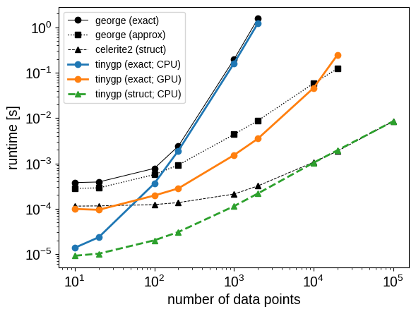
In the plot of this benchmark, you’ll notice several features:

1. For very small datasets, the tinygp CPU implementations are significantly faster than any of the other implementations. This is because jax.jit removes a lot of the Python overhead that is encountered when chaining numpy functions.

2. For medium to large datasets, tinygp is generally faster than george, with the GPU version seeing a significant advantage.

3. The CPU implementations approach the expected asymptotic complexity of \(\mathcal{O}(N^3)\) only for the largest values of \(N\). This is probably caused by memory allocation overhead or other operations with better scaling than the Cholesky factorization.

4. The approximate “HODLR” solver from george outperforms the GPU-enabled tinygp exact solver, but only for very large datasets, and it’s important to note that the HODLR method does not scale well to larger input dimensions. Any existing or future approximate solvers like this that are implemented in jax could be easily used in conjunction with tinygp, but such things have not yet been implemented.

5. The celerite2 and tinygp structured kernel implementation have nearly identical performance for large systems, but the tinygp implementation is significantly faster for small systems (despite being implemented in high-level jax, whereas celerite2 is mostly written in C++).

plt.loglog(
    ns[: len(george_time)],
    george_time,
    "o-",
    color="k",
    lw=0.75,
    label="george (exact)",
)
plt.loglog(
    ns[: len(hodlr_time)],
    hodlr_time,
    "s:",
    color="k",
    lw=1,
    label="george (approx)",
)
plt.loglog(ns, celerite_time, "^--", color="k", lw=0.75, label="celerite2 (struct)")

plt.loglog(
    ns[: len(cpu_time)],
    cpu_time,
    "o-",
    color="C0",
    lw=2,
    label="tinygp (exact; CPU)",
)
plt.loglog(
    ns[: len(gpu_time)],
    gpu_time,
    "o-",
    color="C1",
    lw=2,
    label="tinygp (exact; GPU)",
)
plt.loglog(ns, quasisep_time, "^--", color="C2", lw=2, label="tinygp (struct; CPU)")

plt.legend(fontsize=10)
plt.xlabel("number of data points")
plt.ylabel("runtime [s]");