Show code cell content Hide code cell content

try:
    import tinygp
except ImportError:
    %pip install -q tinygp

try:
    import jaxopt
except ImportError:
    %pip install -q jaxopt

Derivative Observations & Pytree Data

As discussed in Section 9.4 of R&W, it is possible to build a model that incorporates observations of the derivative of the process. In this case, the kernel becomes:

\[ \mathrm{cov}\left(f_i,\, f_j\right) = k(x_i,\,x_j) \]

\[ \mathrm{cov}\left(f_i,\, \dot{f}_j\right) = \frac{\partial k(x_i,\,x_j)}{\partial x_j} \]

\[ \mathrm{cov}\left(\dot{f}_i,\, \dot{f}_j\right) = \frac{\partial k(x_i,\,x_j)}{\partial x_i \partial x_j} \]

where \(\dot{f}_i\) is the derivative of the process at \(x_i\). Since jax can easily compose derivatives, it is straightforward to implement such a model with tinygp.

In this case, our data points will each by a tuple with the x coordinate, and a boolean flag that is True when that observation is of the derivative of the process. An important thing to note here is that the tinygp.kernels.Kernel.evaluate() method always operates on a single pair of inputs. This means that in evaluate, you can unpack (x, flag) = X where x is the input coordinate and flag is a boolean flag.

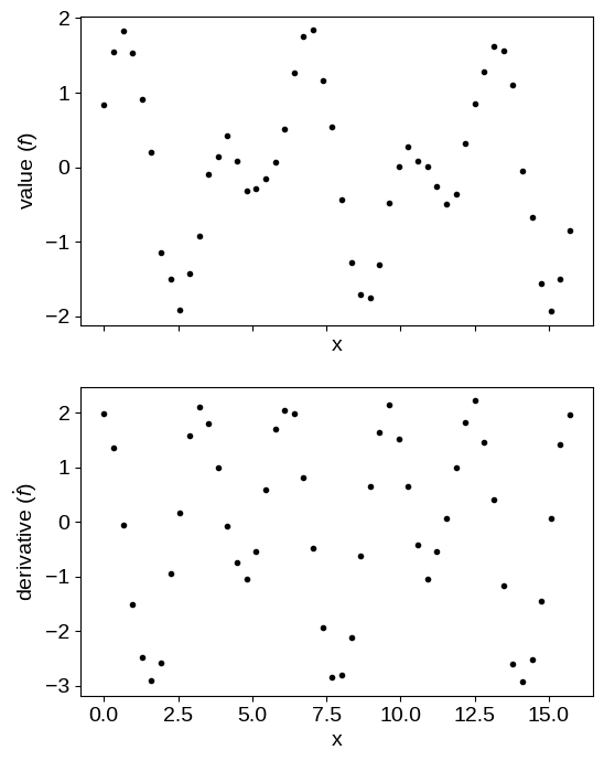
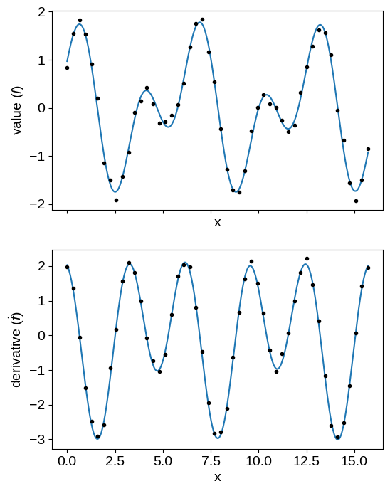
To begin, let’s simulate some data following this example from the GPyTorch documentation:

import numpy as np
import matplotlib.pyplot as plt


X = np.linspace(0.0, 5 * np.pi, 50)
y = np.concatenate(
    (
        np.sin(2 * X) + np.cos(X),
        -np.sin(X) + 2 * np.cos(2 * X),
    )
)
flag = np.concatenate((np.zeros(len(X), dtype=bool), np.ones(len(X), dtype=bool)))
X = np.concatenate((X, X))
y += 0.1 * np.random.default_rng(1234).normal(size=len(y))

fig, axes = plt.subplots(2, 1, figsize=(6, 8), sharex=True)
axes[0].plot(X[~flag], y[~flag], ".k", label="value")
axes[1].plot(X[flag], y[flag], ".k", label="derivative")
axes[0].set_xlabel("x")
axes[1].set_xlabel("x")
axes[0].set_ylabel("value ($f$)")
_ = axes[1].set_ylabel(r"derivative ($\dot{f}$)")

Here’s how we implement the kernel for this model:

import tinygp
import jax
import jax.numpy as jnp

jax.config.update("jax_enable_x64", True)


class DerivativeKernel(tinygp.kernels.Kernel):
    kernel: tinygp.kernels.Kernel

    def evaluate(self, X1, X2):
        t1, d1 = X1
        t2, d2 = X2

        # Differentiate the kernel function: the first derivative wrt x1
        Kp = jax.grad(self.kernel.evaluate, argnums=0)

        # ... and the second derivative
        Kpp = jax.grad(Kp, argnums=1)

        # Evaluate the kernel matrix and all of its relevant derivatives
        K = self.kernel.evaluate(t1, t2)
        d2K_dx1dx2 = Kpp(t1, t2)

        # For stationary kernels, these are related just by a minus sign, but we'll
        # evaluate them both separately for generality's sake
        dK_dx2 = jax.grad(self.kernel.evaluate, argnums=1)(t1, t2)
        dK_dx1 = Kp(t1, t2)

        return jnp.where(
            d1, jnp.where(d2, d2K_dx1dx2, dK_dx1), jnp.where(d2, dK_dx2, K)
        )

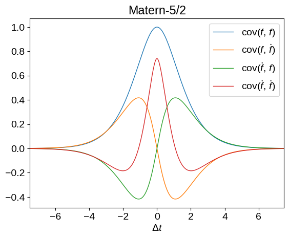
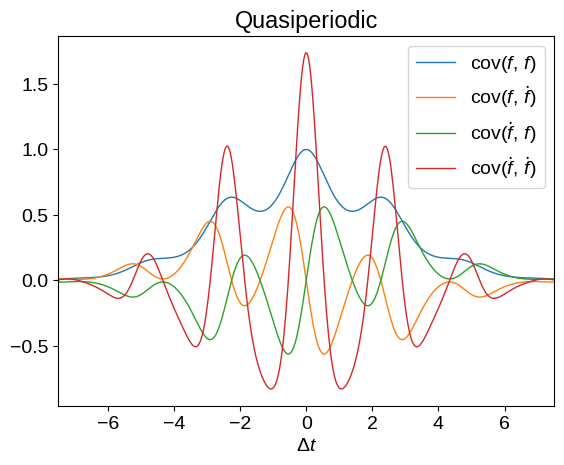
Now that we have this definition, we can plot what the kernel functions look like for different base kernels, \(k(x_i,\,x_j)\) above. Don’t worry too much about the syntax here but, in these plots, we’re showing all the covariances between \(f\) and \(\dot{f}\).

def plot_kernel(base_kernel):
    kernel = DerivativeKernel(base_kernel)

    N = 500
    dt = np.linspace(-7.5, 7.5, N)

    k00 = kernel(
        (jnp.zeros((1)), jnp.zeros((1), dtype=bool)),
        (dt, np.zeros(N, dtype=bool)),
    )[0]
    k11 = kernel(
        (jnp.zeros((1)), jnp.ones((1), dtype=bool)),
        (dt, np.ones(N, dtype=bool)),
    )[0]
    k01 = kernel(
        (jnp.zeros((1)), jnp.zeros((1), dtype=bool)),
        (dt, np.ones(N, dtype=bool)),
    )[0]
    k10 = kernel(
        (jnp.zeros((1)), jnp.ones((1), dtype=bool)),
        (dt, np.zeros(N, dtype=bool)),
    )[0]

    plt.figure()
    plt.plot(dt, k00, label="$\mathrm{cov}(f,\,f)$", lw=1)
    plt.plot(dt, k01, label="$\mathrm{cov}(f,\,\dot{f})$", lw=1)
    plt.plot(dt, k10, label="$\mathrm{cov}(\dot{f},\,f)$", lw=1)
    plt.plot(dt, k11, label="$\mathrm{cov}(\dot{f},\,\dot{f})$", lw=1)
    plt.legend()
    plt.xlabel(r"$\Delta t$")
    plt.xlim(dt.min(), dt.max())


plot_kernel(tinygp.kernels.Matern52(scale=1.5))
plt.title("Matern-5/2")

plot_kernel(
    tinygp.kernels.ExpSquared(scale=2.5)
    * tinygp.kernels.ExpSineSquared(scale=2.5, gamma=0.5)
)
_ = plt.title("Quasiperiodic")

Now we can fit our simulated data using this kernel. Note, especially that we pass in (X, flag) as the input coordinates for the training data.

import jaxopt


def build_gp(params):
    base_kernel = jnp.exp(2 * params["log_amp"]) * tinygp.kernels.ExpSquared(
        scale=jnp.exp(params["log_scale"])
    )
    kernel = DerivativeKernel(base_kernel)

    # Note that we're passing in (X, flag) as the input coordinates.
    return tinygp.GaussianProcess(kernel, (X, flag), diag=jnp.exp(params["log_diag"]))


@jax.jit
def loss(params):
    gp = build_gp(params)
    return -gp.log_probability(y)


init = {
    "log_scale": np.log(1.5),
    "log_amp": np.log(1.0),
    "log_diag": np.log(0.1),
}
print(f"Initial negative log likelihood: {loss(init)}")
solver = jaxopt.ScipyMinimize(fun=loss)
soln = solver.run(init)
print(f"Final negative log likelihood: {soln.state.fun_val}")

Initial negative log likelihood: 98.40600089321084

Final negative log likelihood: -13.27256035026609

X_grid = np.linspace(0, 5 * np.pi, 500)
gp = build_gp(soln.params)

# Predict the function values for the function and its derivative
mu1 = gp.condition(y, (X_grid, np.zeros(len(X_grid), dtype=bool))).gp.loc
mu2 = gp.condition(y, (X_grid, np.ones(len(X_grid), dtype=bool))).gp.loc

fig, axes = plt.subplots(2, 1, figsize=(6, 8), sharex=True)

axes[0].plot(X_grid, mu1)
axes[0].plot(X[~flag], y[~flag], ".k")
axes[1].plot(X_grid, mu2)
axes[1].plot(X[flag], y[flag], ".k", label="derivative")

axes[0].set_xlabel("x")
axes[1].set_xlabel("x")
axes[0].set_ylabel("value ($f$)")
_ = axes[1].set_ylabel(r"derivative ($\dot{f}$)")

A more detailed example: A latent GP & derivative

Building on the previous example, we will next build a custom kernel that is commonly used when studying radial velocity observations of exoplanet-hosting stars, as described by Rajpaul et al. (2015). Take a look at that paper for more details about the math, but the tl;dr is that we want to model a set parallel, but qualitatively different, time series, using a latent Gaussian process. The interesting part of this model is that Rajpaul et al. model the observations as arbitrary linear combinations of the process and its first time derivative, and they work through the derivation of the resulting kernel function.

In this tutorial, we will implement this kernel using tinygp—something that is significantly more annoying to do with other Gaussian process frameworks (trust me, I’ve tried!)—and demonstrate a few key features along the way.

The kernel

The kernel matrix described by Rajpaul et al. (2015) is a block matrix where each element is a linear combination of the latent kernel and its first and second derivatives, where the relevant coefficients depend on the “class” of each pair of observations. This means that our input data needs to include, at each observation, the time t (our input coordinate in this case) and an integer class label label. As above, we will structure our data in such a way that we can treat each input as being a tuple (t, label). In this case, we will unpack our inputs t, label = X and treat t and label as scalars. Here’s our implementation:

class LatentKernel(tinygp.kernels.Kernel):
    """A custom kernel based on Rajpaul et al. (2015)

    Args:
        kernel: The kernel function describing the latent process. This can be any other
            ``tinygp`` kernel.
        coeff_prim: The primal coefficients for each class. This can be thought of as how
            much the latent process itself projects into the observations for that class.
            This should be an array with an entry for each class of observation.
        coeff_deriv: The derivative coefficients for each class. This should have the same
            shape as ``coeff_prim``.
    """

    kernel: tinygp.kernels.Kernel
    coeff_prim: jax.Array
    coeff_deriv: jax.Array

    def __init__(self, kernel, coeff_prim, coeff_deriv):
        self.kernel = kernel
        self.coeff_prim, self.coeff_deriv = jnp.broadcast_arrays(
            jnp.asarray(coeff_prim), jnp.asarray(coeff_deriv)
        )

    def evaluate(self, X1, X2):
        t1, label1 = X1
        t2, label2 = X2

        # Differentiate the kernel function: the first derivative wrt x1
        Kp = jax.grad(self.kernel.evaluate, argnums=0)

        # ... and the second derivative
        Kpp = jax.grad(Kp, argnums=1)

        # Evaluate the kernel matrix and all of its relevant derivatives
        K = self.kernel.evaluate(t1, t2)
        d2K_dx1dx2 = Kpp(t1, t2)

        # For stationary kernels, these are related just by a minus sign, but we'll
        # evaluate them both separately for generality's sake
        dK_dx2 = jax.grad(self.kernel.evaluate, argnums=1)(t1, t2)
        dK_dx1 = Kp(t1, t2)

        # Extract the coefficients
        a1 = self.coeff_prim[label1]
        a2 = self.coeff_prim[label2]
        b1 = self.coeff_deriv[label1]
        b2 = self.coeff_deriv[label2]

        # Construct the matrix element
        return a1 * a2 * K + a1 * b2 * dK_dx2 + b1 * a2 * dK_dx1 + b1 * b2 * d2K_dx1dx2

Inference

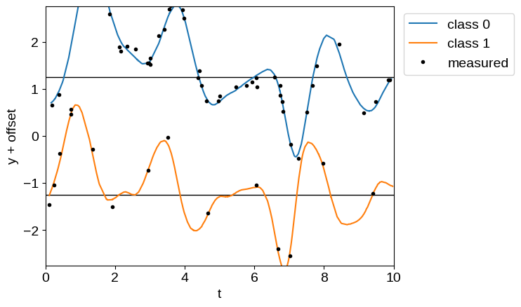
Given this custom kernel definition, let’s simulate some data and fit for the kernel parameters. In this case, we’ll use the product of an kernels.ExpSquared and a kernels.ExpSineSquared kernel for our latent process. Note that we’re not including an amplitude parameter in our latent process, since that will be captured by the coefficients in our LatentKernel defined above. Using this latent process, we simulate an unbalanced dataset with two classes and plot the simulated data below, with class offsets for clarity.

base_kernel = tinygp.kernels.ExpSquared(scale=1.5) * tinygp.kernels.ExpSineSquared(
    scale=2.5, gamma=0.5
)
kernel = LatentKernel(base_kernel, [1.0, 0.5], [-0.1, 0.3])

random = np.random.default_rng(5678)
t1 = np.sort(random.uniform(0, 10, 200))
label1 = np.zeros_like(t1, dtype=int)
t2 = np.sort(random.uniform(0, 10, 300))
label2 = np.ones_like(t2, dtype=int)
X = (np.append(t1, t2), np.append(label1, label2))

gp = tinygp.GaussianProcess(kernel, X, diag=1e-5)
y = gp.sample(jax.random.PRNGKey(1234))

subset = np.append(
    random.integers(len(t1), size=50),
    len(t1) + random.integers(len(t2), size=15),
)
X_obs = (X[0][subset], X[1][subset])
y_obs = y[subset] + 0.1 * random.normal(size=len(subset))

offset = 2.5

plt.axhline(0.5 * offset, color="k", lw=1)
plt.axhline(-0.5 * offset, color="k", lw=1)

plt.plot(t1, y[: len(t1)] + 0.5 * offset, label="class 0")
plt.plot(t2, y[len(t1) :] - 0.5 * offset, label="class 1")

plt.plot(X_obs[0], y_obs + offset * (0.5 - X_obs[1]), ".k", label="measured")

plt.xlim(0, 10)
plt.ylim(-1.1 * offset, 1.1 * offset)
plt.xlabel("t")
plt.ylabel("y + offset")
_ = plt.legend(bbox_to_anchor=(1.01, 1), loc="upper left")

Then, we fit the simulated data, by optimizing for the maximum likelihood kernel parameters using jaxopt:

import jaxopt


def build_gp(params):
    base_kernel = tinygp.kernels.ExpSquared(
        scale=jnp.exp(params["log_scale"])
    ) * tinygp.kernels.ExpSineSquared(
        scale=jnp.exp(params["log_period"]), gamma=params["gamma"]
    )
    kernel = LatentKernel(base_kernel, params["coeff_prim"], params["coeff_deriv"])
    return tinygp.GaussianProcess(kernel, X_obs, diag=jnp.exp(params["log_diag"]))


@jax.jit
def loss(params):
    gp = build_gp(params)
    return -gp.log_probability(y_obs)


init = {
    "log_scale": np.log(1.5),
    "log_period": np.log(2.5),
    "gamma": np.float64(0.5),
    "coeff_prim": np.array([1.0, 0.5]),
    "coeff_deriv": np.array([-0.1, 0.3]),
    "log_diag": np.log(0.1),
}
print(f"Initial negative log likelihood: {loss(init)}")
solver = jaxopt.ScipyMinimize(fun=loss)
soln = solver.run(init)
print(f"Final negative log likelihood: {soln.state.fun_val}")

Initial negative log likelihood: 18.547339999954147

Final negative log likelihood: -20.014003748537824

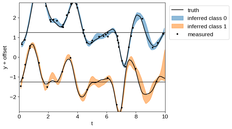
And plot the resulting inference. Of particular note here, even for the sparsely sampled “class 1” dataset, we get robust predictions for the expected process, since we have more finely sampled observations in “class 0”.

gp = build_gp(soln.params)
gp_cond = gp.condition(y_obs, X).gp
mu, var = gp_cond.loc, gp_cond.variance

plt.axhline(0.5 * offset, color="k", lw=1)
plt.axhline(-0.5 * offset, color="k", lw=1)

plt.plot(t1, y[: len(t1)] + 0.5 * offset, "k", label="truth")
plt.plot(t2, y[len(t1) :] - 0.5 * offset, "k")

for c in [0, 1]:
    delta = offset * (0.5 - c)
    m = X[1] == c
    plt.fill_between(
        X[0][m],
        delta + mu[m] + 2 * np.sqrt(var[m]),
        delta + mu[m] - 2 * np.sqrt(var[m]),
        color=f"C{c}",
        alpha=0.5,
        label=f"inferred class {c}",
    )

plt.plot(X_obs[0], y_obs + offset * (0.5 - X_obs[1]), ".k", label="measured")

plt.xlim(0, 10)
plt.ylim(-1.1 * offset, 1.1 * offset)
plt.xlabel("t")
plt.ylabel("y + offset")
_ = plt.legend(bbox_to_anchor=(1.01, 1), loc="upper left")