Show code cell content Hide code cell content

try:
    import tinygp
except ImportError:
    %pip install -q tinygp

try:
    import jaxopt
except ImportError:
    %pip install -q jaxopt

Custom Quasiseparable Kernels

Warning

This implementation of quasiseparable kernels is still experimental, and the models in this tutorial depend on low-level features that are subject to change.

The quasiseparable kernels built in to tinygp are all designed to be used with one-dimensional data (see kernels.quasisep package), but one of the key selling points of the tinygp implementation over other similar projects (e.g. celerite, celerite2, S+LEAF), is that it has a model building interface that is more expressive and flexible. In this tutorial, we present some examples of the kinds of extensions that are possible within this framework. This will be one of the most technical tinygp tutorials, and the implementation details are likely to change in future versions; you have been warned!

Multivariate quasiseparable kernels

Gordon et al. (2020) demonstrated how the celerite algorithm could be extended to model “rectangular” data (e.g. parallel time series), and here we’ll implement a slightly more general model that includes the Gordon et al. (2020) model as a special case. But to start, let’s implement something that is very similar to the simplest model from Gordon et al. (2020). In this model, we have a single underlying Gaussian process, and each data point is generated from that process with a different amplitude. To add a little more structure to the model, we’ll imagine that we’re modeling “multi-band” data where each observation is indexed by “time” (or some other one-dimensional input coordinate) and it’s band ID (an integer).

We’re not going to go into the mathematical details here (stay tuned for more details, or maybe even a publication?), but the methods that our custom kernel needs to overload here are tinygp.kernels.quasisep.Quasisep.coord_to_sortable() and tinygp.kernels.quasisep.Quasisep.observation_model(). The first method (coord_to_sortable) takes our structured input (in this case a tuple with time as the first element, and band ID as the second), and returns a scalar that is sorted in the dataset (in this case, the time coordinate is what we need). The second method (observation_model) is where the magic happens. To get the behavior that we want here, we overload the observation_model by scaling the observation for each data point by the amplitude in that band.

Here’s how we would implement this in tinygp:

import jax
import jax.numpy as jnp

import tinygp

jax.config.update("jax_enable_x64", True)


@tinygp.helpers.dataclass
class Multiband(tinygp.kernels.quasisep.Wrapper):
    amplitudes: jnp.ndarray

    def coord_to_sortable(self, X):
        return X[0]

    def observation_model(self, X):
        return self.amplitudes[X[1]] * self.kernel.observation_model(X[0])

Some notes here:

1. We’re using tinygp.kernels.quasisep.Wrapper as our base class (instead of tinygp.kernels.quasisep.Quasisep), since it provides some help when writing a custom kernel that wraps another quasiseparable kernel.

2. We’ve decorated our class with the @tinygp.helpers.dataclass decorator which, while not strictly necessary, can make our lives a little easier.

Now that we have this implementation, let’s build an example model with a tinygp.kernels.quasisep.Matern52 as our base kernel and 3 bands. Then we’ll sample from it to get a sense for what is going on:

Show code cell content Hide code cell content

def plot_multiband_sample(kernel):
    gp = tinygp.GaussianProcess(kernel, X)
    y = gp.sample(jax.random.PRNGKey(849))
    for i in np.unique(band_id):
        plt.axhline(-7 * i, color="k")
        plt.plot(t[band_id == i], y[band_id == i] - 7 * i, label=f"band {i + 1}")
    plt.xlim(0, 10)
    plt.ylim(-21, 7)
    plt.yticks([])
    plt.xlabel("x")
    plt.ylabel("y + offset")
    plt.legend(fontsize=10, loc=2)

import numpy as np
import matplotlib.pyplot as plt

random = np.random.default_rng(394)
t = np.sort(random.uniform(0, 10, 700))
band_id = random.choice([0, 1, 2], size=len(t))
X = (t, band_id)

kernel = Multiband(
    kernel=tinygp.kernels.quasisep.Matern52(scale=1.5),
    amplitudes=jnp.array([3.1, -1.1, 3.7]),
)

plot_multiband_sample(kernel)

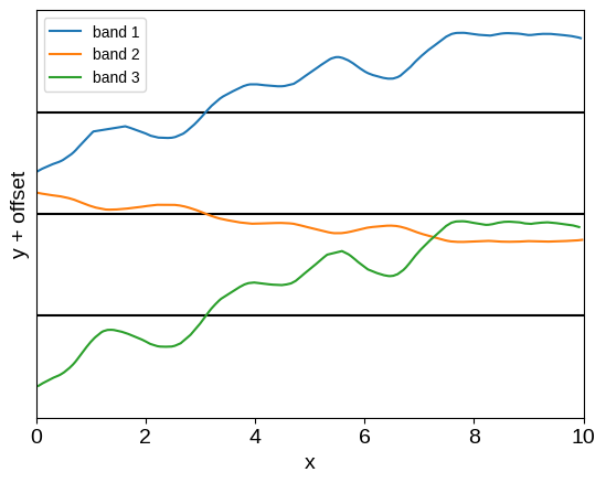
This model is very similar to the baseline model introduced by Gordon et al. (2020; their Equation 13), with the added generalization that we’re not restricted to rectangular data: the observations don’t need to be simultaneous. While Gordon et al. (2020) showed that this model could be useful, it’s not actually very expressive, so let’s take another step.

The most obvious generalization of this simple model is to take the sum of several Multiband kernels with different amplitudes and, optionally, different underlying processes. As an example, here’s what happens if we take the sum of two of our custom kernels:

kernel = Multiband(
    kernel=tinygp.kernels.quasisep.Matern52(scale=1.5),
    amplitudes=jnp.array([0.9, 0.7, -1.1]),
)
kernel += Multiband(
    kernel=tinygp.kernels.quasisep.Matern52(scale=0.5),
    amplitudes=jnp.array([1.1, -1.7, 1.5]),
)
plot_multiband_sample(kernel)

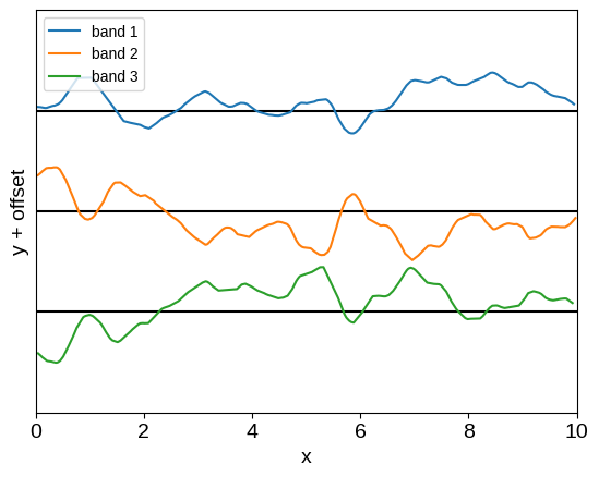
This is already a much more expressive kernel, with some shared structure between the two bands, but this relationship is much less restrictive.

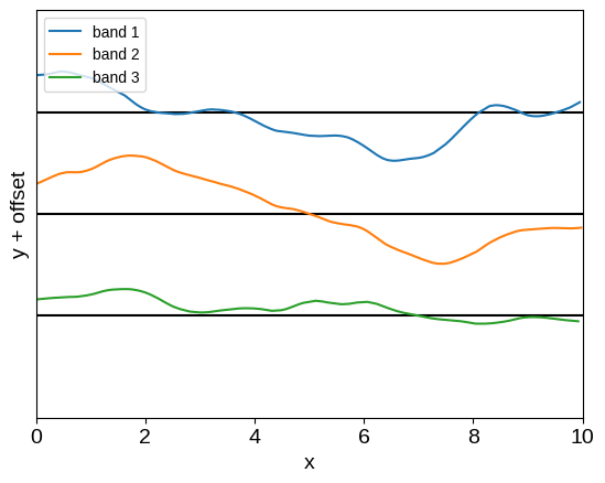
We can also reproduce the full-rank Kronecker model from Gordon et al. (2020) using this same infrastructure. In that case, we need to sum the same number of Multiband kernels as there are bands, using the same baseline kernel for each. Then, if we call the \(N_\mathrm{band} \times N_\mathrm{band}\) cross-band covariance matrix \(R\) following Gordon et al. (2020), and take its Cholesky factorization \(R = L\,L^\mathrm{T}\), the amplitude for the \(n\)-th term is the \(n\)-th row of \(L\). For example, we could use an exponential-squared kernel for the cross-band band covariance:

R = 1.5**2 * jnp.exp(-0.5 * (jnp.arange(3)[:, None] - jnp.arange(3)[None, :]) ** 2)
L = jnp.linalg.cholesky(R)

base_kernel = tinygp.kernels.quasisep.Matern52(scale=1.5)
kernel = sum(Multiband(kernel=base_kernel, amplitudes=row) for row in L)
plot_multiband_sample(kernel)

And now we have a flexible and expressive, but still scalable, kernel for analyzing multi-band data. While we have captured the models studied by Gordon et al. (2020) as special cases, the framework proposed here presents several nice generalizations to those results:

1. These models are no longer restricted to rectangular data where every band is observed at every time,

2. This conceptually different approach where we model the data using a mixture of latent processes, observed using linear projections, permits a wider range of modeling choices, and may be useful for incorporating physical knowledge/interpretation into the model.

Quasiseparable kernels & derivative observations

Recently, Delisle et al. (2022) demonstrated that models of derivative observations (like the ones discussed in the Derivative Observations & Pytree Data tutorial) could also be implemented using the celerite algorithm, without increasing the order of the model. In this example, we demonstrate how such processes can be implemented in tinygp. While the resulting model here is qualitatively similar to that introduced by Delisle et al. (2022), the technical implementation details are substantially different, but we’ll leave our discussion to the details to a future publication.

As our demonstration of this type of modeling, we will roughly reproduce the example described in the A more detailed example: A latent GP & derivative section of the Derivative Observations & Pytree Data tutorial, so you should check that out first if you haven’t already.

To implement that model in tinygp, we will again base our model on the tinygp.kernels.quasisep.Wrapper base class, and overload the coord_to_sortable and observation_model methods. Because of how these quasiseparable kernels are implemented, the derivative model is actually significantly simpler to implement than the general case discussed in A more detailed example: A latent GP & derivative, but you’ll just have to trust us on this for now until we can reference the technical details elsewhere.

Here’s our implementation:

@tinygp.helpers.dataclass
class Latent(tinygp.kernels.quasisep.Wrapper):
    coeff_prim: jnp.ndarray
    coeff_deriv: jnp.ndarray

    def coord_to_sortable(self, X):
        return X[0]

    def observation_model(self, X):
        t, label = X
        design = self.kernel.design_matrix()
        obs = self.kernel.observation_model(t)
        obs_prim = jnp.asarray(self.coeff_prim)[label] * obs
        obs_deriv = jnp.asarray(self.coeff_deriv)[label] * obs @ design
        return obs_prim - obs_deriv


base_kernel = tinygp.kernels.quasisep.Matern52(
    scale=1.5
) * tinygp.kernels.quasisep.Cosine(scale=2.5)
kernel = Latent(base_kernel, [0.5, 0.02], [0.01, -0.2])

# Unlike the previous derivative observations tutorial, the datapoints here
# must be sorted in time.
random = np.random.default_rng(5678)
t = np.sort(random.uniform(0, 10, 500))
label = (random.uniform(0, 1, len(t)) < 0.5).astype(int)
X = (t, label)

gp = tinygp.GaussianProcess(kernel, X)
y = gp.sample(jax.random.PRNGKey(12345))

# Select a subset of the data as "observations"
subset = (1 + 2 * label) * random.uniform(0, 1, len(t)) < 0.3
X_obs = (X[0][subset], X[1][subset])
y_obs = y[subset] + 0.1 * random.normal(size=subset.sum())

offset = 2.5

plt.axhline(0.5 * offset, color="k", lw=1)
plt.axhline(-0.5 * offset, color="k", lw=1)
plt.plot(t[label == 0], y[label == 0] + 0.5 * offset, label="class 0")
plt.plot(t[label == 1], y[label == 1] - 0.5 * offset, label="class 1")
plt.plot(X_obs[0], y_obs + offset * (0.5 - X_obs[1]), ".k", label="measured")

plt.xlim(0, 10)
plt.ylim(-1.3 * offset, 1.3 * offset)
plt.xlabel("t")
plt.ylabel("y + offset")
_ = plt.legend(bbox_to_anchor=(1.01, 1), loc="upper left")

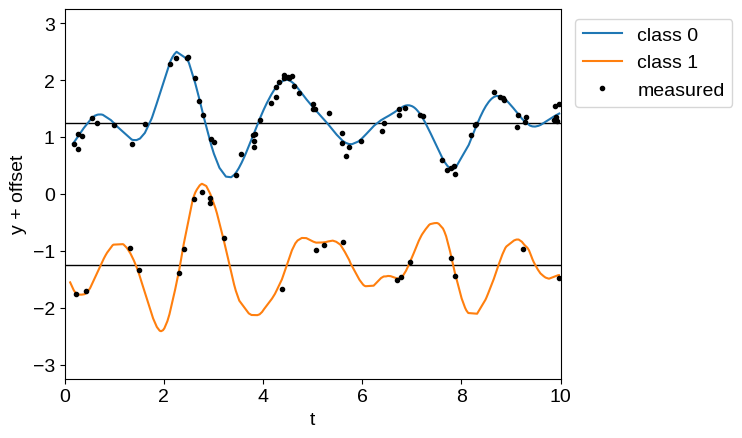
There are a few things that are worth noting here. First, unlike in the Derivative Observations & Pytree Data tutorial, our data must be correctly ordered (in this case by t). This is true for any quasiseparable model, but it isn’t going to be checked; you’ll just end up with a lot of NaNs.

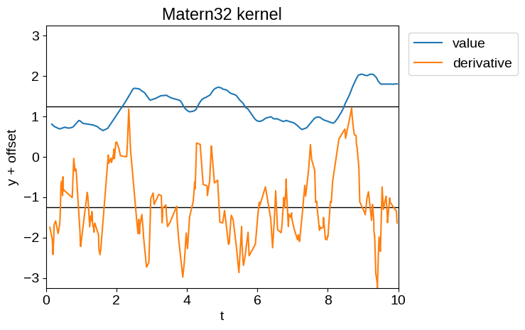
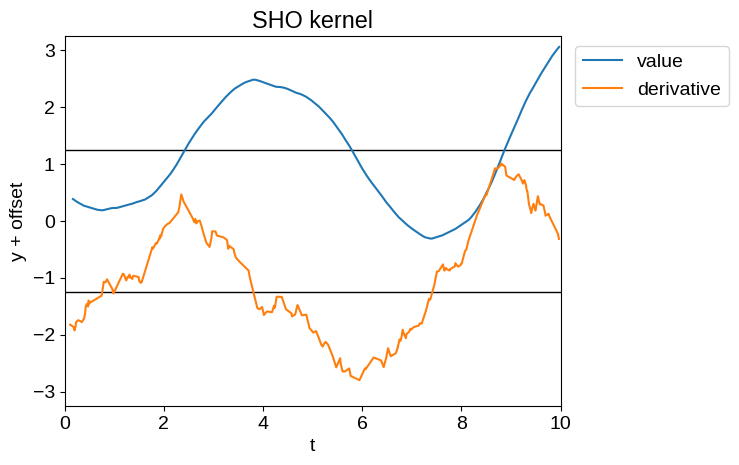
Second, let’s take a brief aside into kernel choices here. Not all the kernels defined in the kernels.quasisep package make sensible choices for problems like this. Some of them (e.g. tinygp.kernels.quasisep.Celerite) are not actually differentiable for all values of their parameters. Others may be differentiable, but their derivative processes may not be well-behaved. For example, the time derivative of a Matern-3/2 process (tinygp.kernels.quasisep.Matern32), or a simple harmonic oscillator process (tinygp.kernels.quasisep.SHO), while defined, will be unphysically noisy as demonstrated below. Therefore, while Delisle et al. (2022) advocated for the use of a mixture of SHO kernels, we don’t recommend that choice.

Show code cell content Hide code cell content

def plot_latent_samples(kernel):
    yp = tinygp.GaussianProcess(
        Latent(kernel, coeff_prim=[1.0, 0.0], coeff_deriv=[0.0, 1.0]), X
    ).sample(jax.random.PRNGKey(12345))

    plt.figure()
    plt.axhline(0.5 * offset, color="k", lw=1)
    plt.axhline(-0.5 * offset, color="k", lw=1)
    plt.plot(t[label == 0], yp[label == 0] + 0.5 * offset, label="value")
    plt.plot(t[label == 1], yp[label == 1] - 0.5 * offset, label="derivative")

    plt.xlim(0, 10)
    plt.ylim(-1.3 * offset, 1.3 * offset)
    plt.xlabel("t")
    plt.ylabel("y + offset")
    _ = plt.legend(bbox_to_anchor=(1.01, 1), loc="upper left")

plot_latent_samples(tinygp.kernels.quasisep.Matern32(1.0, sigma=0.5))
plt.title("Matern32 kernel")

plot_latent_samples(tinygp.kernels.quasisep.SHO(quality=10.0, omega=1.0))
_ = plt.title("SHO kernel")

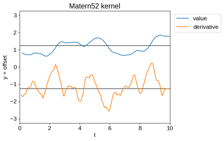
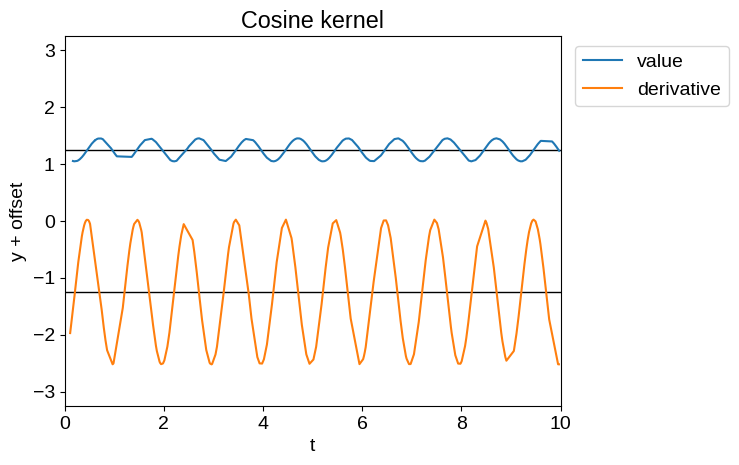
Of the kernels currently implemented in the kernels.quasisep package, the most sensible ones for our purposes are tinygp.kernels.quasisep.Matern52, tinygp.kernels.quasisep.Cosine, and sums and products thereof. Samples of these processes and their derivatives are shown below:

plot_latent_samples(tinygp.kernels.quasisep.Matern52(1.0, sigma=0.5))
plt.title("Matern52 kernel")

plot_latent_samples(tinygp.kernels.quasisep.Cosine(1.0, sigma=0.2))
_ = plt.title("Cosine kernel")

Now that we’ve been through this aside, let’s get back to fitting our simulated data from above. In this case we’ll model the data using the same model that we used to simulate it: the product of a Matern52 kernel and a Cosine kernel.

import jaxopt


def build_gp(params):
    base_kernel = tinygp.kernels.quasisep.Matern52(
        scale=jnp.exp(params["log_scale"])
    ) * tinygp.kernels.quasisep.Cosine(scale=jnp.exp(params["log_period"]))
    kernel = Latent(base_kernel, params["coeff_prim"], params["coeff_deriv"])
    return tinygp.GaussianProcess(kernel, X_obs, diag=jnp.exp(params["log_diag"]))


@jax.jit
def loss(params):
    gp = build_gp(params)
    return -gp.log_probability(y_obs)


init = {
    "log_scale": np.log(1.5),
    "log_period": np.log(2.5),
    "coeff_prim": np.array([0.5, 0.02]),
    "coeff_deriv": np.array([0.01, -0.2]),
    "log_diag": np.log(0.1),
}
print(f"Initial negative log likelihood: {loss(init)}")
solver = jaxopt.ScipyMinimize(fun=loss)
soln = solver.run(init)
print(f"Final negative log likelihood: {soln.state.fun_val}")

Initial negative log likelihood: 9.56314077667156

Final negative log likelihood: -51.40561724640375

Having optimized our model, we can plot the model predictions and compare them to the true model:

gp = build_gp(soln.params)
gp_cond = gp.condition(y_obs, X).gp
mu, var = gp_cond.loc, gp_cond.variance

plt.axhline(0.5 * offset, color="k", lw=1)
plt.axhline(-0.5 * offset, color="k", lw=1)

plt.plot(t[label == 0], y[label == 0] + 0.5 * offset, "k", label="truth")
plt.plot(t[label == 1], y[label == 1] - 0.5 * offset, "k")

for c in [0, 1]:
    delta = offset * (0.5 - c)
    m = X[1] == c
    plt.fill_between(
        X[0][m],
        delta + mu[m] + 2 * np.sqrt(var[m]),
        delta + mu[m] - 2 * np.sqrt(var[m]),
        color=f"C{c}",
        alpha=0.5,
        label=f"inferred class {c}",
    )

plt.plot(X_obs[0], y_obs + offset * (0.5 - X_obs[1]), ".k", label="measured")

plt.xlim(0, 10)
plt.ylim(-1.1 * offset, 1.1 * offset)
plt.xlabel("t")
plt.ylabel("y + offset")
_ = plt.legend(bbox_to_anchor=(1.01, 1), loc="upper left")

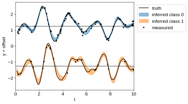
Like in the A more detailed example: A latent GP & derivative tutorial, even though we have many fewer observations of “class 1”, we are still able to make good predictions for its behavior by propagating information from the observations of “class 0”.

Quasiseparable kernels with banded observation models

This example doesn’t directly fit in this tutorial since we’re not implementing a custom kernel, but without a better place to put it we wanted to mention that the tinygp.noise.Banded observation noise model is fully compatible with the tinygp.solvers.quasisep.QuasisepSolver. The fact that this works stems from the fact that banded matrices can be exactly represented as quasiseparable matrices (see tinygp.noise.Banded for more details).

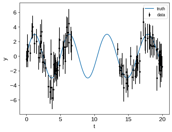
This means that it is also possible to implement the class of models supported by the S+LEAF package using tinygp. To demonstrate this, we can roughly reproduce this example from the S+LEAF documentation. First, we generate a simulated data that is similar to the one from that example:

Show code cell content Hide code cell content

random = np.random.default_rng(0)

nt = 100
tmax = 20
t = np.sort(
    np.concatenate(
        (
            random.uniform(0, tmax / 3, nt // 2),
            random.uniform(2 * tmax / 3, tmax, (nt + 1) // 2),
        )
    )
)

# Quasiperiodic signal
amp = 3.0
P0 = 5.2
dP = 0.75
P = P0 + dP * (t / tmax - 1 / 2)
y = amp * np.sin(2 * np.pi * t / P)
tsmooth = np.linspace(0, tmax, 2000)
Psmooth = P0 + dP * (tsmooth / tmax - 1 / 2)
ysignal = amp * np.sin(2 * np.pi * tsmooth / Psmooth)
dysignal = (
    amp
    * 2
    * np.pi
    / Psmooth
    * (1 - tsmooth * dP / (tmax * Psmooth))
    * np.cos(2 * np.pi * tsmooth / Psmooth)
)

# Measurement noise
yerr_meas = random.uniform(0.5, 1.5, nt)
y = y + random.normal(0, yerr_meas)

# Calibration noise
calib_id = (t // 1).astype(int)
caliberr = random.uniform(0.5, 1.5, calib_id[-1] + 1)
yerr_calib = caliberr[calib_id]
y += random.normal(0, caliberr)[calib_id]

yerr = np.sqrt(yerr_meas**2 + yerr_calib**2)
plt.plot(tsmooth, ysignal, label="truth")
plt.errorbar(t, y, yerr, fmt=".", color="k", label="data")
plt.xlabel("t")
plt.ylabel("y")
_ = plt.legend(fontsize=10)

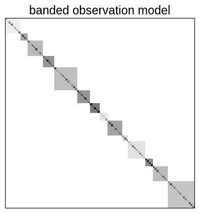
Then, we can build the band matrix representation of the observation process. In this case, this is a block diagonal matrix, and here’s one way that you might construct it:

from collections import Counter

bandwidth = max(Counter(calib_id).values()) - 1
off_diags = np.zeros((nt, bandwidth))
for j in range(bandwidth):
    m = calib_id[: nt - j - 1] == calib_id[j + 1 :]
    off_diags[: nt - j - 1, j][m] = caliberr[calib_id[: nt - j - 1][m]] ** 2

noise_model = tinygp.noise.Banded(diag=yerr**2, off_diags=off_diags)

plt.imshow(noise_model @ np.eye(nt), cmap="gray_r")
plt.xticks([])
plt.yticks([])
_ = plt.title("banded observation model")

Then we can use this noise model to fit for the parameters of our model. It would also be possible to fit for the elements of this band matrix by just computing the indices above, instead of the full noise model, but for simplicity we’ll just keep the noise model fixed for this example.

import jaxopt


def build_gp(params):
    kernel = tinygp.kernels.quasisep.SHO(
        sigma=jnp.exp(params["log_sigma"]),
        quality=jnp.exp(params["log_quality"]),
        omega=jnp.exp(params["log_omega"]),
    )
    return tinygp.GaussianProcess(kernel, t, noise=noise_model)


@jax.jit
def loss(params):
    gp = build_gp(params)
    return -gp.log_probability(y)


init = {
    "log_sigma": jnp.log(0.5),
    "log_quality": jnp.log(5.0),
    "log_omega": jnp.zeros(()),
}
print(f"Initial negative log likelihood: {loss(init)}")
solver = jaxopt.ScipyMinimize(fun=loss)
soln = solver.run(init)
print(f"Final negative log likelihood: {soln.state.fun_val}")

# Plot the results
gp = build_gp(soln.params)
gp_cond = gp.condition(y, tsmooth).gp
mu, var = gp_cond.loc, gp_cond.variance
std = np.sqrt(var)

plt.plot(tsmooth, ysignal, label="truth")
plt.errorbar(t, y, yerr, fmt=".", color="k", label="data")
plt.plot(tsmooth, mu, color="C1", label="predicted")
plt.fill_between(tsmooth, mu - std, mu + std, color="C1", alpha=0.3)
plt.xlabel("t")
plt.ylabel("y")
_ = plt.legend(fontsize=10)

Initial negative log likelihood: 194.75537378078377

Final negative log likelihood: 171.1410280586686

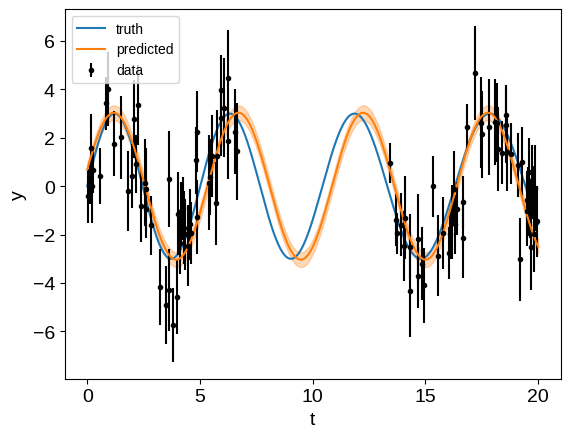
Like in the S+LEAF docs, if we were to restrict ourselves to a diagonal noise model our interpolated results wouldn’t be great, but when we take them into account, the predictions aren’t too bad.