Show code cell content Hide code cell content

try:
    import tinygp
except ImportError:
    %pip install -q tinygp

try:
    import jaxopt
except ImportError:
    %pip install -q jaxopt

Fitting a Mean Function

It is quite common in the GP literature to (“without lack of generality”) set the mean of the process to zero and call it a day. In practice, however, it is often useful to fit for the parameters of a mean model at the same time as the GP parameters. In some other tutorials, we fit for a constant mean value using the mean argument to tinygp.GaussianProcess, but in this tutorial we walk through an example for how you might go about fitting a model with a non-trival parameterized mean function.

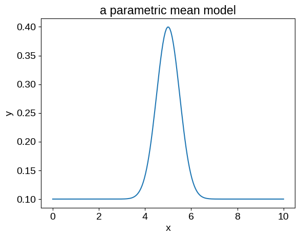
For our example, we’ll fit for the location, width, and amplitude of the following model:

\[ f(x) = b + a\,\exp\left(-\frac{(x - \ell)^2}{2\,w^2}\right) \]

In jax, we might implement such a function as follows:

from functools import partial
import numpy as np
import matplotlib.pyplot as plt
import jax
import jax.numpy as jnp

jax.config.update("jax_enable_x64", True)


def mean_function(params, X):
    mod = jnp.exp(-0.5 * jnp.square((X - params["loc"]) / jnp.exp(params["log_width"])))
    beta = jnp.array([1, mod])
    return params["amps"] @ beta


mean_params = {
    "amps": np.array([0.1, 0.3]),
    "loc": 5.0,
    "log_width": np.log(0.5),
}

X_grid = np.linspace(0, 10, 200)
model = jax.vmap(partial(mean_function, mean_params))(X_grid)

plt.plot(X_grid, model)
plt.xlabel("x")
plt.ylabel("y")
_ = plt.title("a parametric mean model")

Our implementation here is somewhat artificially complicated in order to highlight one very important technical point: we must define our mean function to operate on a single input coordinate. What that means is that we don’t need to worry about broadcasting and stuff within our mean function: tinygp will do all the necessary vmap-ing. More explicitly, if we try to call our mean_function on a vector of inputs, it will fail with a strange error (yeah, I know that we could write it in a way that would work, but I’m trying to make a point!):

model = mean_function(mean_params, X_grid)

---------------------------------------------------------------------------
ValueError                                Traceback (most recent call last)
Cell In[3], line 1
----> 1 model = mean_function(mean_params, X_grid)

Cell In[2], line 12, in mean_function(params, X)
     10 def mean_function(params, X):
     11     mod = jnp.exp(-0.5 * jnp.square((X - params["loc"]) / jnp.exp(params["log_width"])))
---> 12     beta = jnp.array([1, mod])
     13     return params["amps"] @ beta

File ~/checkouts/readthedocs.org/user_builds/tinygp/envs/stable/lib/python3.10/site-packages/jax/_src/numpy/lax_numpy.py:2158, in array(object, dtype, copy, order, ndmin)
   2156 elif isinstance(object, (list, tuple)):
   2157   if object:
-> 2158     out = stack([asarray(elt, dtype=dtype) for elt in object])
   2159   else:
   2160     out = np.array([], dtype=dtype)  # type: ignore[arg-type]

File ~/checkouts/readthedocs.org/user_builds/tinygp/envs/stable/lib/python3.10/site-packages/jax/_src/numpy/lax_numpy.py:1839, in stack(arrays, axis, out, dtype)
   1837 for a in arrays:
   1838   if shape(a) != shape0:
-> 1839     raise ValueError("All input arrays must have the same shape.")
   1840   new_arrays.append(expand_dims(a, axis))
   1841 return concatenate(new_arrays, axis=axis, dtype=dtype)

ValueError: All input arrays must have the same shape.

Instead, we need to manually vmap as follows:

model = jax.vmap(partial(mean_function, mean_params))(X_grid)

Simulated data

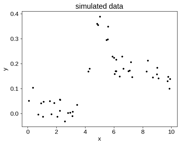
Now that we have this mean function defined, let’s make some fake data that could benefit from a joint GP + mean function fit. In this case, we’ll add a background trend that’s not included in the mean model, as well as some noise.

random = np.random.default_rng(135)
X = np.sort(random.uniform(0, 10, 50))
y = jax.vmap(partial(mean_function, mean_params))(X)
y += 0.1 * np.sin(2 * np.pi * (X - 5) / 10.0)
y += 0.03 * random.normal(size=len(X))
plt.plot(X, y, ".k")
plt.xlabel("x")
plt.ylabel("y")
_ = plt.title("simulated data")

The fit

Then, we set up the usual infrastructure to calculate the loss function for this model. In this case, you’ll notice that we’ve stacked the mean and GP parameters into one dictionary, but that isn’t the only way you could do it. You’ll also notice that we’re passing a partially evaluated version of the mean function to our GP object, but we’re not doing any vmap-ing. That’s because tinygp is expecting the mean function to operate on a single input coordinate, and it will handle the appropriate mapping.

from tinygp import kernels, GaussianProcess


def build_gp(params):
    kernel = jnp.exp(params["log_gp_amp"]) * kernels.Matern52(
        jnp.exp(params["log_gp_scale"])
    )
    return GaussianProcess(
        kernel,
        X,
        diag=jnp.exp(params["log_gp_diag"]),
        mean=partial(mean_function, params),
    )


@jax.jit
def loss(params):
    gp = build_gp(params)
    return -gp.log_probability(y)


params = dict(
    log_gp_amp=np.log(0.1),
    log_gp_scale=np.log(3.0),
    log_gp_diag=np.log(0.03),
    **mean_params,
)
loss(params)

Array(-33.08457135, dtype=float64)

We can minimize the loss using jaxopt:

import jaxopt

solver = jaxopt.ScipyMinimize(fun=loss)
soln = solver.run(jax.tree_util.tree_map(jnp.asarray, params))
print(f"Final negative log likelihood: {soln.state.fun_val}")

Final negative log likelihood: -99.26464900290122

Visualizing result

And then plot the conditional distribution:

gp = build_gp(soln.params)
_, cond = gp.condition(y, X_grid)

mu = cond.loc
std = np.sqrt(cond.variance)

plt.plot(X, y, ".k", label="data")
plt.plot(X_grid, mu, label="model")
plt.fill_between(X_grid, mu + std, mu - std, color="C0", alpha=0.3)

plt.xlim(X_grid.min(), X_grid.max())
plt.xlabel("x")
plt.ylabel("y")
_ = plt.legend()

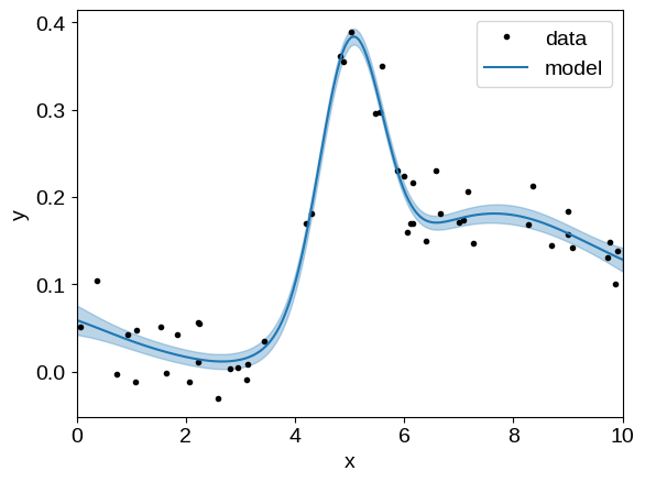
That looks pretty good but, when working with mean functions, it is often useful to separate the mean model and GP predictions when plotting the conditional. The interface for doing this in tinygp is not its most ergonomic feature, but it shouldn’t be too onerous. To compute the conditional distribution, without the mean function included, call tinygp.GaussianProcess.condition() with the include_mean=False flag:

gp = build_gp(soln.params)
_, cond = gp.condition(y, X_grid, include_mean=False)

mu = cond.loc + soln.params["amps"][0]
std = np.sqrt(cond.variance)

plt.plot(X, y, ".k", label="data")
plt.plot(X_grid, mu, label="GP model")
plt.fill_between(X_grid, mu + std, mu - std, color="C0", alpha=0.3)
plt.plot(X_grid, jax.vmap(gp.mean_function)(X_grid), label="mean model")

plt.xlim(X_grid.min(), X_grid.max())
plt.xlabel("x")
plt.ylabel("y")
_ = plt.legend()

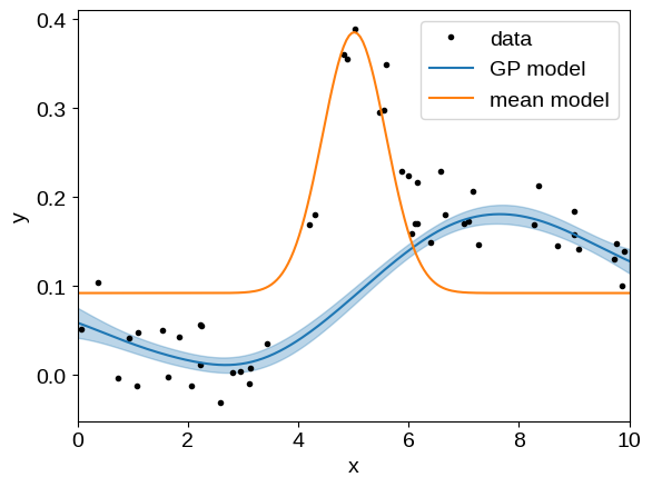
There is one other subtlety that you may notice here: we added the mean model’s zero point (params["amps"][0]) to the GP prediction. If we had left this off, the blue line in the above figure would be offset below the data by about 0.1, and it’s pretty common that you’ll end up with a workflow like this when visualizing the results of GP fits with non-trivial means.

An alternative workflow

Sometimes it can be easier to manage all the mean function bookkeeping yourself, and instead of using the mean argument to tinygp.GaussianProcess, you could instead manually subtract the mean function from the data before calling tinygp.GaussianProcess.log_probability(). Here’s how you might implement such a workflow for our example:

vmapped_mean_function = jax.vmap(mean_function, in_axes=(None, 0))


def build_gp_v2(params):
    kernel = jnp.exp(params["log_gp_amp"]) * kernels.Matern52(
        jnp.exp(params["log_gp_scale"])
    )
    return GaussianProcess(kernel, X, diag=jnp.exp(params["log_gp_diag"]))


@jax.jit
def loss_v2(params):
    gp = build_gp_v2(params)
    return -gp.log_probability(y - vmapped_mean_function(params, X))


loss_v2(params)

Array(-33.08457135, dtype=float64)

In this case, we are now responsible for making sure that the mean function is properly broadcasted, and we must not forget to also subtract the mean function when calling tinygp.GaussianProcess.condition().