Show code cell content Hide code cell content

try:
    import tinygp
except ImportError:
    %pip install -q tinygp

try:
    import jaxopt
except ImportError:
    %pip install -q jaxopt

Getting Started

Note

This tutorial will introduce some of the basic usage of tinygp, but since we’re going to be leaning pretty heavily on jax, it might be useful to also take a look at the jax docs for some more basic introduction to jax programming patterns.

In the following, we’ll reproduce the analysis for Figure 5.6 in Chapter 5 of Rasmussen & Williams (R&W). The data are measurements of the atmospheric CO2 concentration made at Mauna Loa, Hawaii (Keeling & Whorf 2004). The dataset is said to be available online but I couldn’t seem to download it from the original source. Luckily the statsmodels package includes a copy that we can load as follows:

import numpy as np
import matplotlib.pyplot as plt
from statsmodels.datasets import co2

data = co2.load_pandas().data
t = 2000 + (np.array(data.index.to_julian_date()) - 2451545.0) / 365.25
y = np.array(data.co2)
m = np.isfinite(t) & np.isfinite(y) & (t < 1996)
t, y = t[m][::4], y[m][::4]

plt.plot(t, y, ".k")
plt.xlim(t.min(), t.max())
plt.xlabel("year")
_ = plt.ylabel("CO$_2$ in ppm")

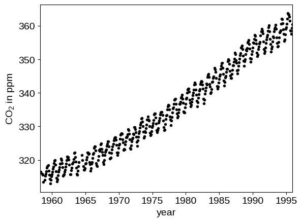
In this figure, you can see that there is periodic (or quasi-periodic) signal with a year-long period superimposed on a long term trend. We will follow R&W and model these effects non-parametrically using a complicated covariance function. The covariance function that we’ll use is:

\[k(r) = k_1(r) + k_2(r) + k_3(r) + k_4(r)\]

where

\[\begin{split} \begin{eqnarray} k_1(r) &=& \theta_1^2 \, \exp \left(-\frac{r^2}{2\,\theta_2} \right) \\ k_2(r) &=& \theta_3^2 \, \exp \left(-\frac{r^2}{2\,\theta_4} -\theta_5\,\sin^2\left( \frac{\pi\,r}{\theta_6}\right) \right) \\ k_3(r) &=& \theta_7^2 \, \left [ 1 + \frac{r^2}{2\,\theta_8\,\theta_9} \right ]^{-\theta_8} \\ k_4(r) &=& \theta_{10}^2 \, \exp \left(-\frac{r^2}{2\,\theta_{11}} \right) + \theta_{12}^2\,\delta_{ij} \end{eqnarray} \end{split}\]

We can implement this kernel in tinygp as follows (we’ll use the R&W results as the hyperparameters for now):

import jax
import jax.numpy as jnp

from tinygp import kernels, GaussianProcess


jax.config.update("jax_enable_x64", True)


def build_gp(theta, X):
    # We want most of our parameters to be positive so we take the `exp` here
    # Note that we're using `jnp` instead of `np`
    amps = jnp.exp(theta["log_amps"])
    scales = jnp.exp(theta["log_scales"])

    # Construct the kernel by multiplying and adding `Kernel` objects
    k1 = amps[0] * kernels.ExpSquared(scales[0])
    k2 = (
        amps[1]
        * kernels.ExpSquared(scales[1])
        * kernels.ExpSineSquared(
            scale=jnp.exp(theta["log_period"]),
            gamma=jnp.exp(theta["log_gamma"]),
        )
    )
    k3 = amps[2] * kernels.RationalQuadratic(
        alpha=jnp.exp(theta["log_alpha"]), scale=scales[2]
    )
    k4 = amps[3] * kernels.ExpSquared(scales[3])
    kernel = k1 + k2 + k3 + k4

    return GaussianProcess(
        kernel, X, diag=jnp.exp(theta["log_diag"]), mean=theta["mean"]
    )


def neg_log_likelihood(theta, X, y):
    gp = build_gp(theta, X)
    return -gp.log_probability(y)


theta_init = {
    "mean": np.float64(340.0),
    "log_diag": np.log(0.19),
    "log_amps": np.log([66.0, 2.4, 0.66, 0.18]),
    "log_scales": np.log([67.0, 90.0, 0.78, 1.6]),
    "log_period": np.float64(0.0),
    "log_gamma": np.log(4.3),
    "log_alpha": np.log(1.2),
}

# `jax` can be used to differentiate functions, and also note that we're calling
# `jax.jit` for the best performance.
obj = jax.jit(jax.value_and_grad(neg_log_likelihood))

print(f"Initial negative log likelihood: {obj(theta_init, t, y)[0]}")
print(
    f"Gradient of the negative log likelihood, wrt the parameters:\n{obj(theta_init, t, y)[1]}"
)

Initial negative log likelihood: 392.9423118570187
Gradient of the negative log likelihood, wrt the parameters:
{'log_alpha': Array(3.3025811, dtype=float64), 'log_amps': Array([-56.37950097,   1.71669126,   4.11084749,  -2.13098285], dtype=float64), 'log_diag': Array(60.28268107, dtype=float64), 'log_gamma': Array(12.52278878, dtype=float64), 'log_period': Array(2339.70173767, dtype=float64), 'log_scales': Array([117.65693454,  -3.10865356, -27.13290445,  -4.04980878], dtype=float64), 'mean': Array(-0.15787706, dtype=float64)}

Some things to note here:

1. If you’re new to jax the way that I’m mixing np and jnp (the jax version of numpy) might seem a little confusing. In this example, I’m using regular numpy to simulate and prepare our test dataset, and then using jax.numpy everywhere else. The important point is that within the neg_log_likelihood function (and all the functions it calls), np is never used.

2. This pattern of writing a build_gp function is a pretty common workflow in these docs. It’s useful to have a way of instantiating our GP model at a new set of parameters, as we’ll see below when we plot the conditional model. This might seem a little strange if you’re coming from other libraries (like george, for example), but if you jit the function (see below) each model evaluation won’t actually instantiate all these classes so you don’t need to worry about performance implications. Check out Modeling Frameworks for some alternative workflows.

3. Make sure that you remember to wrap your function in jax.jit. The jax docs have more details about how this works, but for our purposes, the key thing is that this allows us to use the expressive tinygp kernel building syntax without worrying about the performance costs of all of these allocations.

Using our loss function defined above, we’ll run a gradient based optimization routine from jaxopt to fit this model as follows:

import jaxopt

solver = jaxopt.ScipyMinimize(fun=neg_log_likelihood)
soln = solver.run(theta_init, X=t, y=y)
print(f"Final negative log likelihood: {soln.state.fun_val}")

Final negative log likelihood: 296.59832192675833

Warning: An optimization code something like this should work on most problems but the results can be very sensitive to your choice of initialization and algorithm. If the results are nonsense, try choosing a better initial guess or try a different value of the method parameter in jaxopt.ScipyMinimize.

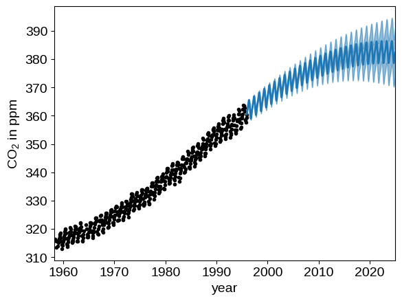
We can plot our prediction of the CO2 concentration into the future using our optimized Gaussian process model by running:

x = np.linspace(max(t), 2025, 2000)
gp = build_gp(soln.params, t)
cond_gp = gp.condition(y, x).gp
mu, var = cond_gp.loc, cond_gp.variance

plt.plot(t, y, ".k")
plt.fill_between(x, mu + np.sqrt(var), mu - np.sqrt(var), color="C0", alpha=0.5)
plt.plot(x, mu, color="C0", lw=2)

plt.xlim(t.min(), 2025)
plt.xlabel("year")
_ = plt.ylabel("CO$_2$ in ppm")