
Custom Geometry#
When working with multivariate inputs, you’ll always need to choose a metric for computing the distance between coordinates in your input space.
As discussed in Multivariate Data, tinygp includes built-in support for some common metrics which, when combined with Kernel Transforms, can cover a wide range of use cases.
But this tutorial covers a more general use case: custom geometries.
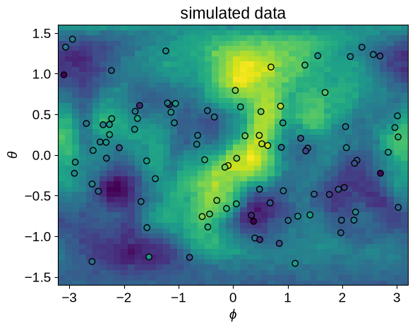
In this example, we will fit a GP model to data that lives on the surface of a sphere. Here, we want to use our knowledge of this system to design a metric that takes this geometry into account. Specifically, our data will have unit vector coordinates, and we will define a great-circle distance to compute the angular distances between these vectors.
import jax
import jax.numpy as jnp
import matplotlib.pyplot as plt
import numpy as np

from tinygp import GaussianProcess, kernels

jax.config.update("jax_enable_x64", True)


class GreatCircleDistance(kernels.stationary.Distance):
    def distance(self, X1, X2):
        if jnp.shape(X1) != (3,) or jnp.shape(X2) != (3,):
            raise ValueError(
                "The great-circle distance is only defined for unit 3-vector"
            )
        return jnp.arctan2(jnp.linalg.norm(jnp.cross(X1, X2)), (X1.T @ X2))


# Make a spherical grid
phi = np.linspace(-np.pi, np.pi, 50)
theta = np.linspace(-0.5 * np.pi, 0.5 * np.pi, 50)
phi_grid, theta_grid = np.meshgrid(phi, theta, indexing="ij")
phi_grid = phi_grid.flatten()
theta_grid = theta_grid.flatten()
X_grid = np.vstack(
    (
        np.cos(phi_grid) * np.cos(theta_grid),
        np.sin(phi_grid) * np.cos(theta_grid),
        np.sin(theta_grid),
    )
).T

# Choose some uniformly distributed coordinates to be our "data"
random = np.random.default_rng(456)
X_obs = random.normal(size=(100, 3))
X_obs /= np.sqrt(np.sum(X_obs**2, axis=1))[:, None]
theta_obs = np.arctan2(X_obs[:, 2], np.sqrt(X_obs[:, 0] ** 2 + X_obs[:, 1] ** 2))
phi_obs = np.arctan2(X_obs[:, 1], X_obs[:, 0])

# Our kernel is parameterized by a length scale in **radians**
ell = 0.5
kernel = 1.5 * kernels.Matern52(ell, distance=GreatCircleDistance())

# Sample a simulated dataset
gp = GaussianProcess(kernel, np.concatenate((X_grid, X_obs), axis=0), diag=0.01)
y_samp = gp.sample(jax.random.PRNGKey(10))
y_grid = y_samp[: len(X_grid)]
y_obs = y_samp[len(X_grid) :] + 0.5 * random.normal(size=len(X_obs))

# Plot the map
plt.pcolor(
    phi,
    theta,
    y_grid.reshape((len(phi), len(theta))).T,
    vmin=y_grid.min(),
    vmax=y_grid.max(),
)
plt.scatter(
    phi_obs,
    theta_obs,
    c=y_obs,
    edgecolor="k",
    vmin=y_grid.min(),
    vmax=y_grid.max(),
)
plt.xlabel(r"$\phi$")
plt.ylabel(r"$\theta$")
_ = plt.title("simulated data")
Using these simulated data, we can now fit the model as usual:
import jaxopt


def build_gp(params):
    kernel = jnp.exp(params["log_amp"]) * kernels.Matern52(
        jnp.exp(params["log_scale"]), distance=GreatCircleDistance()
    )
    return GaussianProcess(
        kernel,
        X_obs,
        diag=jnp.exp(2 * params["log_sigma"]),
        mean=params["mean"],
    )


@jax.jit
def loss(params):
    return -build_gp(params).log_probability(y_obs)


params = {
    "log_amp": np.zeros(()),
    "log_scale": np.zeros(()),
    "log_sigma": np.zeros(()),
    "mean": np.zeros(()),
}
solver = jaxopt.ScipyMinimize(fun=loss)
soln = solver.run(params)
gp = build_gp(soln.params)
At the maximum point, we can plot our model prediction compared to the ground truth, with the residuals plotted on the same scale:
y_pred = gp.condition(y_obs, X_grid).gp.loc

fig, axes = plt.subplots(3, 1, sharex=True, figsize=(8, 8))

axes[0].set_title("truth")
axes[0].pcolor(
    phi,
    theta,
    y_grid.reshape((len(phi), len(theta))).T,
    vmin=y_grid.min(),
    vmax=y_grid.max(),
)

axes[1].set_title("predicted")
axes[1].pcolor(
    phi,
    theta,
    y_pred.reshape((len(phi), len(theta))).T,
    vmin=y_grid.min(),
    vmax=y_grid.max(),
)

axes[2].set_title("residuals")
axes[2].pcolor(
    phi,
    theta,
    (y_pred - y_grid).reshape((len(phi), len(theta))).T,
    vmin=y_grid.min(),
    vmax=y_grid.max(),
)

axes[2].set_xlabel(r"$\phi$")
for ax in axes:
    ax.set_ylabel(r"$\theta$")
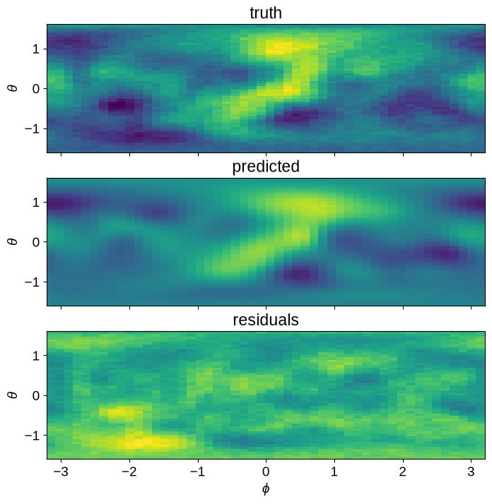
One thing that is worth commenting on here is that, unlike in Multivariate Data, we’re using only a single length scale. This means that our kernel is isotropic. For many use cases this is probably what you want because the whole point of this distance metric is that it is rotationally invariant. If you want to model or discover anisotropies, you could use the methods discussed in Kernel Transforms, but it would probably be worth considering designing a kernel that better captures what you’re trying to model.