Show code cell content Hide code cell content

try:
    import tinygp
except ImportError:
    %pip install -q tinygp

An Introduction to tinygp

This tutorial provides a brief introduction to how Gaussian Processes (GPs) are implemented in tinygp. We’re not going to provide much of an introduction to GPs themselves, because there are already a lot of excellent resources for that, including this text book, this blog post, and many others that I’m sure you can find by Googling.

Before we get started, it’s pretty much always a good idea to enable double precision before doing anything with tinygp and GPs in jax, so that we end up with fewer numerical precision issues:

import jax

jax.config.update("jax_enable_x64", True)

Kernel building

In tinygp, we primarily construct GP models, by specifying a “kernel” function defined using the building blocks in the kernels package. For example, we can define an “exponential squared” or “radial basis function” kernel using:

from tinygp import kernels

kernel = kernels.ExpSquared(scale=1.5)

And we can plot its value (don’t worry too much about the syntax here):

import numpy as np
import matplotlib.pyplot as plt


def plot_kernel(kernel, **kwargs):
    dx = np.linspace(0, 5, 100)
    plt.plot(dx, kernel(dx, dx[:1]), **kwargs)
    plt.xlabel("dx")
    plt.ylabel("k(dx)")


plot_kernel(kernel)

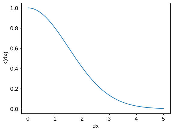
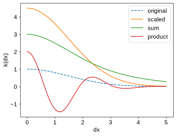
This kernel on its own is not terribly expressive, so we’ll usually end up adding and multiplying kernels to build the function we want. For example, we can:

• scale our kernel by a scalar,

• add multiple different kernels, or

• multiply kernels together

as follows:

plot_kernel(kernel, label="original", ls="dashed")

kernel_scaled = 4.5 * kernels.ExpSquared(scale=1.5)
plot_kernel(kernel_scaled, label="scaled")

kernel_sum = kernels.ExpSquared(scale=1.5) + 2 * kernels.Matern32(scale=2.5)
plot_kernel(kernel_sum, label="sum")

kernel_prod = 2 * kernels.ExpSquared(scale=1.5) * kernels.Cosine(scale=2.5)
plot_kernel(kernel_prod, label="product")

_ = plt.legend()

For a lot of use cases, these operations will be sufficient to build the models that you need, but if not, check out the following tutorials for some more expressive examples: Custom Kernels, Kernel Transforms, Custom Geometry, and Derivative Observations & Pytree Data.

Sampling

Once you have a kernel in hand, you can pass it to a tinygp.GaussianProcess to handle most of the computations you need. The tinygp.GaussianProcess will also need to know the input coordinates of your data X (let’s just make some up for now) and it takes a little parameter diag, which specifies extra variance to add on the diagonal. When modeling real data, this can often be thought of as per-observation measurement uncertainty, but it may not always be obvious what to put there. That being said, you’ll probably find that if you don’t use the diag parameter you’ll get a lot of nans in your results, so it’s generally good to at least provide some small value for diag.

from tinygp import GaussianProcess

# Let's make up some input coordinates (sorted for plotting purposes)
X = np.sort(np.random.default_rng(1).uniform(0, 10, 100))

gp = GaussianProcess(kernel, X)

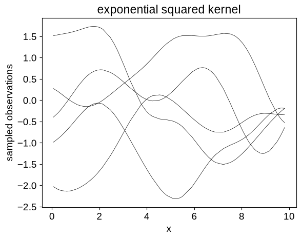
This gp object now specifies a multivariate normal distribution over data points observed at X. It’s sometimes useful to generate samples from this distribution to see what our prior looks like. We can do that using the GaussianProcess.sample() function, and this will be the first time we’re going to need to do anything jax-specific (because of how random numbers work in jax):

y = gp.sample(jax.random.PRNGKey(4), shape=(5,))
plt.plot(X, y.T, color="k", lw=0.5)
plt.xlabel("x")
plt.ylabel("sampled observations")
_ = plt.title("exponential squared kernel")

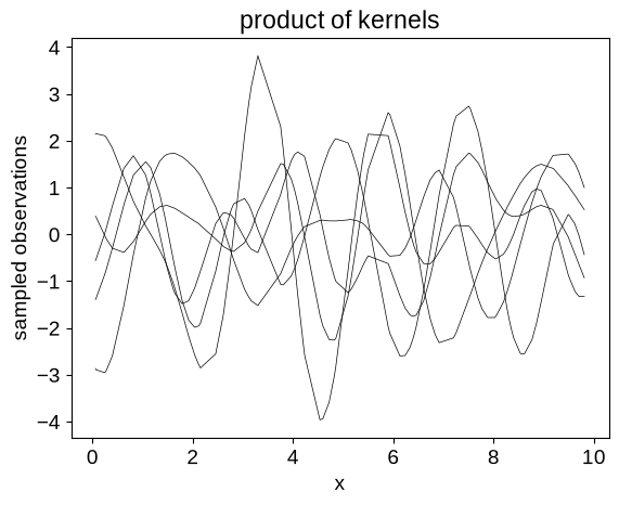
We can also generate samples for different kernel functions:

# Here we're using the product of kernels defined above
kernel_prod = 2 * kernels.ExpSquared(scale=1.5) * kernels.Cosine(scale=2.5)
gp = GaussianProcess(kernel_prod, X, diag=1e-5)
y = gp.sample(jax.random.PRNGKey(4), shape=(5,))

plt.plot(X, y.T, color="k", lw=0.5)
plt.xlabel("x")
plt.ylabel("sampled observations")
_ = plt.title("product of kernels")

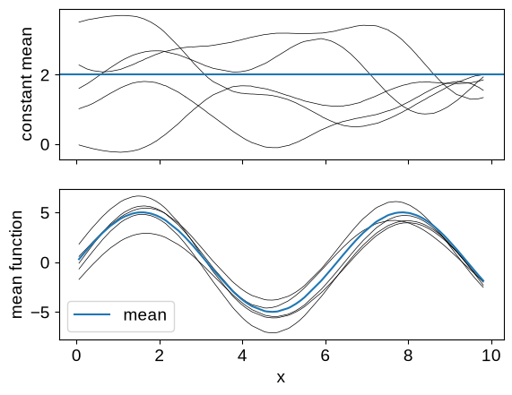
It is quite common in the GP literature to set the mean function for our process to zero, but that isn’t always what you want. Instead, you can set the mean to a different constant, or to a function:

# A GP with a non-zero constant mean
gp = GaussianProcess(kernel, X, diag=1e-5, mean=2.0)
y_const = gp.sample(jax.random.PRNGKey(4), shape=(5,))


# And a GP with a general mean function
def mean_function(x):
    return 5 * jax.numpy.sin(x)


gp = GaussianProcess(kernel, X, diag=1e-5, mean=mean_function)
y_func = gp.sample(jax.random.PRNGKey(4), shape=(5,))

# Plotting these samples
_, axes = plt.subplots(2, 1, sharex=True)
ax = axes[0]
ax.plot(X, y_const.T, color="k", lw=0.5)
ax.axhline(2.0)
ax.set_ylabel("constant mean")

ax = axes[1]
ax.plot(X, y_func.T, color="k", lw=0.5)
ax.plot(X, jax.vmap(mean_function)(X), label="mean")
ax.legend()
ax.set_xlabel("x")
_ = ax.set_ylabel("mean function")

Conditioning & marginalization

When it comes time to fit data using a GP model, the key operations that tinygp provides are conditioning and marginalization. For example, you may want to fit for the parameters of your kernel model (the length scale and amplitude, for example), and a good objective to use for that process is the marginal likelihood of the process evaluated for the observed data. In tinygp, this is accessed via the tinygp.GaussianProcess.log_probability() method, which takes the observed data y as input. (Aside: The nomenclature for this method is a little tricky to get right, and we’ve settled on log_probability in tinygp since it is the multivariate normal probability density, but it’s important to remember that it is a function of the data, making it a “sampling distribution” or “likelihood”.) We won’t actually go into details about how to use this method for fitting here (check out pretty much any of the other tutorials for examples!), but to compute the log probability for a given dataset and kernel, we would do something like the following:

# Simulate a made up dataset, as an example
random = np.random.default_rng(1)
X = np.sort(random.uniform(0, 10, 10))
y = np.sin(X) + 1e-4 * random.normal(size=X.shape)

# Compute the log probability
kernel = 0.5 * kernels.ExpSquared(scale=1.0)
gp = GaussianProcess(kernel, X, diag=1e-4)
print(gp.log_probability(y))

0.1646203249131255

But we do want to go into more details about how tinygp implements conditioning because it might be a little counterintuitive at first (and it’s also different in v0.2 of tinygp). To condition a GP on observed data, we use the tinygp.GaussianProcess.condition() method, and that produces a named tuple with two elements as described in tinygp.gp.ConditionResult. The first element log_probability is the same log probability as we calculated above:

cond = gp.condition(y)
print(cond.log_probability)

0.1646203249131255

Then the second element gp is a new tinygp.GaussianProcess describing the distribution at some test points (by default, the test points are the same as our inputs). This conditioned GP operates just like our gp above, but its kernel and mean_function have these strange types:

type(cond.gp.kernel), type(cond.gp.mean_function)

(tinygp.kernels.base.Conditioned, tinygp.means.Conditioned)

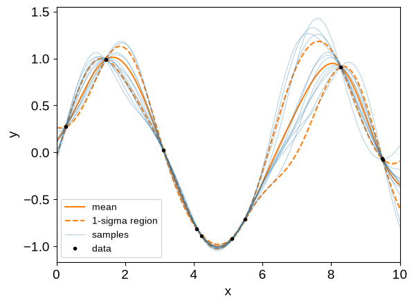
This is cool because that means that you can use this conditioned tinygp.GaussianProcess to do all the things you would usually do with a GP (e.g. sample from it, condition it further, etc.). It is common to make plots like the following using these conditioned GPs (note that we’re now using different test points):

X_test = np.linspace(0, 10, 100)
_, cond_gp = gp.condition(y, X_test)

# The GP object keeps track of its mean and variance, which we can use for
# plotting confidence intervals
mu = cond_gp.mean
std = np.sqrt(cond_gp.variance)
plt.plot(X_test, mu, "C1", label="mean")
plt.plot(X_test, mu + std, "--C1", label="1-sigma region")
plt.plot(X_test, mu - std, "--C1")

# We can also plot samples from the conditional
y_samp = cond_gp.sample(jax.random.PRNGKey(1), shape=(12,))
plt.plot(X_test, y_samp[0], "C0", lw=0.5, alpha=0.5, label="samples")
plt.plot(X_test, y_samp[1:].T, "C0", lw=0.5, alpha=0.5)

plt.plot(X, y, ".k", label="data")
plt.legend(fontsize=10)
plt.xlim(X_test.min(), X_test.max())
plt.xlabel("x")
_ = plt.ylabel("y")

Tips

Given the information we’ve covered so far, you may have just about everything you need to go on to the other tutorials, and start using tinygp for real. But there were a few last things that are worth mentioning first.

First, since tinygp is built on top of jax, it can be very useful to spend some time learning about jax, and in particular the How to Think in JAX tutorial is a great place to start. One way that this plays out in tinygp, is that all the operations described in this tutorial are designed to be jit compiled, rather than executed directly like we’ve done here. Specifically, a very common pattern that you’ll see is a functional model setup like the following:

import jax.numpy as jnp


def build_gp(params):
    kernel = jnp.exp(params["log_amp"]) * kernels.ExpSquared(
        jnp.exp(params["log_scale"])
    )
    return GaussianProcess(kernel, X, diag=jnp.exp(params["log_diag"]))


@jax.jit
def loss(params):
    gp = build_gp(params)
    return -gp.log_probability(y)


params = {
    "log_amp": -0.1,
    "log_scale": 0.0,
    "log_diag": -1.0,
}
loss(params)

Array(10.26490546, dtype=float64)

This is a good setup because the build_gp function can be reused for conditioning the GP, but the @jax.jit decorator on loss means that jax can optimize out all the Python overhead introduced by instantiating the kernel and gp objects.

Finally, the Troubleshooting page includes some other tips for dealing with issues that you might run into, but you should also be encouraged to open issues on the tinygp GitHub repo if you run into other problems.