
Scalable GPs with Quasiseparable Kernels#
Warning
The algorithms described in this section are inherently serial, and you will probably see extremely degraded performance if you turn on GPU acceleration.
Starting with v0.2, tinygp includes an experimental pure-jax implementation of the algorithms behind the celerite package.
The celerite2 package already had support for jax, but since it doesn’t depend on any extra compiled code, the implementation here in tinygp might be a little easier to get up and running, and it is significantly more flexible.
Similarly, even though it is implemented directly in jax, instead of highly-optimized C++ code, the tinygp implementation has similar performance to the celerite2 version (see Benchmarks).
All this being said, this performance doesn’t come for free. In particular, this solver can only be used with data with sortable inputs, and specific types of kernels. In practice this generally means that you’ll need 1-D input data (e.g. a time series) and you’ll need to build your kernel using the members of the kernels.quasisep package. But, if your problem has this form, you may see several orders of magnitude improvement in the runtime of you model.
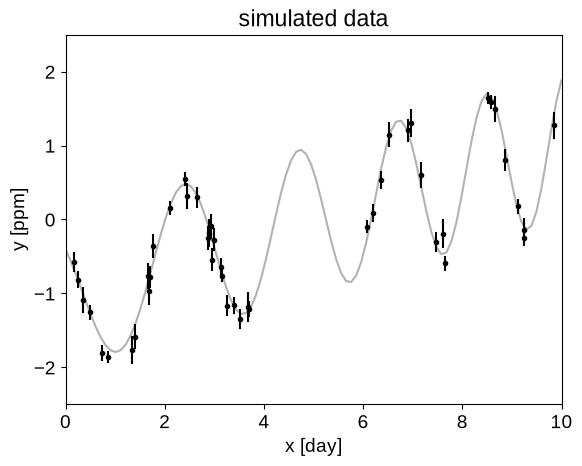
As a demonstration, let’s use the same sample dataset as we used in Modeling Frameworks tutorial:
import matplotlib.pyplot as plt
import numpy as np

random = np.random.default_rng(42)

t = np.sort(
    np.append(
        random.uniform(0, 3.8, 28),
        random.uniform(5.5, 10, 18),
    )
)
yerr = random.uniform(0.08, 0.22, len(t))
y = (
    0.2 * (t - 5)
    + np.sin(3 * t + 0.1 * (t - 5) ** 2)
    + yerr * random.normal(size=len(t))
)

true_t = np.linspace(0, 10, 100)
true_y = 0.2 * (true_t - 5) + np.sin(3 * true_t + 0.1 * (true_t - 5) ** 2)

plt.plot(true_t, true_y, "k", lw=1.5, alpha=0.3)
plt.errorbar(t, y, yerr=yerr, fmt=".k", capsize=0)
plt.xlabel("x [day]")
plt.ylabel("y [ppm]")
plt.xlim(0, 10)
plt.ylim(-2.5, 2.5)
_ = plt.title("simulated data")
Then we can set up our scalable GP model.
This looks (perhaps deceivingly) similar to the model set up that we would normally use, but all the kernels that we’re using are defined in tinygp.kernels.quasisep, instead of tinygp.kernels.
These kernels do, however, still support addition, multiplication, and scaling to build expressive models.
That being said, it’s important to point out that the computational cost of these methods scales poorly with the number of kernels that you add or (worse!) multiply.
import jax
import jax.numpy as jnp

from tinygp import GaussianProcess, kernels

jax.config.update("jax_enable_x64", True)


def build_gp(params):
    kernel = kernels.quasisep.SHO(
        sigma=jnp.exp(params["log_sigma1"]),
        omega=jnp.exp(params["log_omega"]),
        quality=jnp.exp(params["log_quality"]),
    )
    kernel += jnp.exp(2 * params["log_sigma2"]) * kernels.quasisep.Matern32(
        scale=jnp.exp(params["log_scale"])
    )
    return GaussianProcess(
        kernel,
        t,
        diag=yerr**2 + jnp.exp(params["log_jitter"]),
        mean=params["mean"],
    )


@jax.jit
def loss(params):
    gp = build_gp(params)
    return -gp.log_probability(y)


params = {
    "mean": 0.0,
    "log_jitter": 0.0,
    "log_sigma1": 0.0,
    "log_omega": np.log(2 * np.pi),
    "log_quality": 0.0,
    "log_sigma2": 0.0,
    "log_scale": 0.0,
}
loss(params)
Array(61.8065268, dtype=float64)
Good - we got a value for our loss function.
We can check that this was actually using the scalable solver defined in tinygp.solvers.quasisep.solver.QuasisepSolver by checking the type of the solver property of our GP:
type(build_gp(params).solver)
tinygp.solvers.quasisep.solver.QuasisepSolver
Now we can minimize the loss:
import jaxopt

solver = jaxopt.ScipyMinimize(fun=loss)
soln = solver.run(jax.tree_util.tree_map(jnp.asarray, params))
print(f"Final negative log likelihood: {soln.state.fun_val}")
Final negative log likelihood: 3.7920344745170205
And plot our results:
_, cond = build_gp(soln.params).condition(y, true_t)

mu = cond.loc
std = np.sqrt(cond.variance)

plt.plot(true_t, true_y, "k", lw=1.5, alpha=0.3, label="truth")
plt.errorbar(t, y, yerr=yerr, fmt=".k", capsize=0)
plt.plot(true_t, mu, label="max likelihood model")
plt.fill_between(true_t, mu + std, mu - std, color="C0", alpha=0.3)
plt.xlabel("x [day]")
plt.ylabel("y [ppm]")
plt.xlim(0, 10)
plt.ylim(-2.5, 2.5)
plt.legend()
_ = plt.title("maximum likelihood")
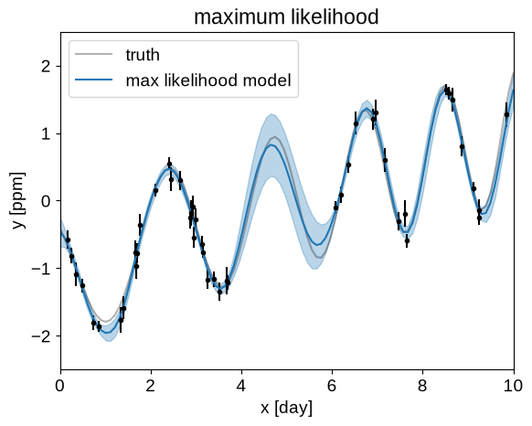
This all looks pretty good!
Before closing out this tutorial, here are some technical details to keep in mind when using this solver:
This implementation is new, and it hasn’t yet been pushed to its limits. If you run into problems, please open issues or pull requests.
The computation of the general conditional model with these kernels is not (yet!) as fast as we might want, and it may be somewhat memory heavy. For very large datasets, it is sometimes sufficient to (a) just compute the conditional at the input points (by omitting the
X_testparameter intinygp.GaussianProcess.condition()), (b) only compute the mean prediction, which should be fast, or (c) only predict at a few test points.For more technical details about these methods, check out the API docs for the kernels.quasisep package, and the solvers.quasisep package, as well as the links therein.
It should be possible to implement more flexible models using this interface than those supported by
celeriteorcelerite2, so stay tuned for more tutorials!