Show code cell content Hide code cell content

try:
    import tinygp
except ImportError:
    %pip install -q tinygp

try:
    import optax
except ImportError:
    %pip install -q optax

Custom Kernels

One of the goals of the tinygp interface design was to make the kernel building framework flexible and easily extensible. In this tutorial, we demonstrate this interface using the “spectral mixture kernel” proposed by Gordon Wilson & Adams (2013). It would be possible to implement this using sums of built-in kernels, but the interface seems better if we implement a custom kernel and I expect that we’d get somewhat better performance for mixtures with many components.

Now, let’s implement this kernel in a way that tinygp understands. When doing this, you will subclass tinygp.kernels.Kernel and implement the tinygp.kernels.Kernel.evaluate() method. One very important thing to note here is that evaluate will always be called via vmap, so you should write your evaluate method to operate on a single pair of inputs and let vmap handle the broadcasting sematics for you.

import tinygp
import jax
import jax.numpy as jnp


class SpectralMixture(tinygp.kernels.Kernel):
    weight: jax.Array
    scale: jax.Array
    freq: jax.Array

    def evaluate(self, X1, X2):
        tau = jnp.atleast_1d(jnp.abs(X1 - X2))[..., None]
        return jnp.sum(
            self.weight
            * jnp.prod(
                jnp.exp(-2 * jnp.pi**2 * tau**2 / self.scale**2)
                * jnp.cos(2 * jnp.pi * self.freq * tau),
                axis=0,
            )
        )

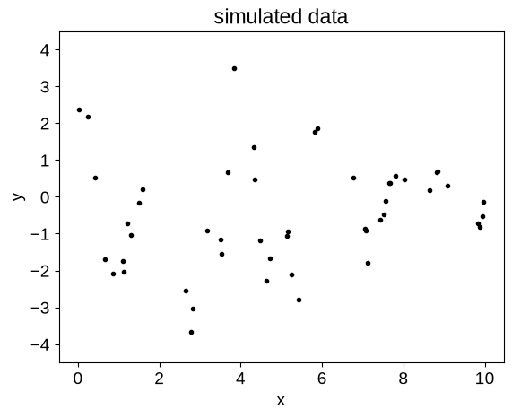
Now let’s implement the simulate some data from this model:

import numpy as np
import matplotlib.pyplot as plt


def build_gp(theta):
    kernel = SpectralMixture(
        jnp.exp(theta["log_weight"]),
        jnp.exp(theta["log_scale"]),
        jnp.exp(theta["log_freq"]),
    )
    return tinygp.GaussianProcess(
        kernel, t, diag=jnp.exp(theta["log_diag"]), mean=theta["mean"]
    )


params = {
    "log_weight": np.log([1.0, 1.0]),
    "log_scale": np.log([10.0, 20.0]),
    "log_freq": np.log([1.0, 1.0 / 2.0]),
    "log_diag": np.log(0.1),
    "mean": 0.0,
}

random = np.random.default_rng(546)
t = np.sort(random.uniform(0, 10, 50))
true_gp = build_gp(params)
y = true_gp.sample(jax.random.PRNGKey(123))

plt.plot(t, y, ".k")
plt.ylim(-4.5, 4.5)
plt.title("simulated data")
plt.xlabel("x")
_ = plt.ylabel("y")

One thing to note here is that we’ve used named parameters in a dictionary, instead of an array of parameters as in some other examples. This would be awkward (but not impossible) to fit using scipy, so instead we’ll use optax for optimization:

import optax


@jax.jit
@jax.value_and_grad
def loss(theta):
    return -build_gp(theta).log_probability(y)


opt = optax.sgd(learning_rate=3e-4)
opt_state = opt.init(params)
for i in range(1000):
    loss_val, grads = loss(params)
    updates, opt_state = opt.update(grads, opt_state)
    params = optax.apply_updates(params, updates)

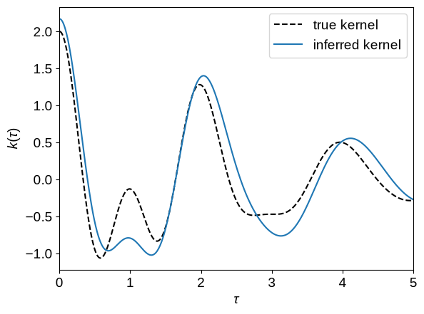
opt_gp = build_gp(params)
tau = np.linspace(0, 5, 500)
plt.plot(tau, true_gp.kernel(tau[:1], tau)[0], "--k", label="true kernel")
plt.plot(tau, opt_gp.kernel(tau[:1], tau)[0], label="inferred kernel")
plt.legend()
plt.xlabel(r"$\tau$")
plt.ylabel(r"$k(\tau)$")
_ = plt.xlim(tau.min(), tau.max())

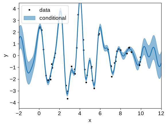
Using our optimized model, over-plot the conditional predictions:

x = np.linspace(-2, 12, 500)
plt.plot(t, y, ".k", label="data")
gp_cond = opt_gp.condition(y, x).gp
mu, var = gp_cond.loc, gp_cond.variance
plt.fill_between(
    x,
    mu + np.sqrt(var),
    mu - np.sqrt(var),
    color="C0",
    alpha=0.5,
    label="conditional",
)
plt.plot(x, mu, color="C0", lw=2)
plt.xlim(x.min(), x.max())
plt.ylim(-4.5, 4.5)
plt.legend(loc=2)
plt.xlabel("x")
_ = plt.ylabel("y")