Show code cell content Hide code cell content

try:
    import tinygp
except ImportError:
    %pip install -q tinygp

try:
    import numpyro
except ImportError:
    %pip uninstall -y jax jaxlib
    %pip install -q numpyro jax jaxlib

try:
    import arviz
except ImportError:
    %pip install arviz

try:
    import flax
except ImportError:
    %pip install -q flax

try:
    import optax
except ImportError:
    %pip install -q optax

/home/docs/checkouts/readthedocs.org/user_builds/tinygp/envs/latest/lib/python3.10/site-packages/tqdm/auto.py:21: TqdmWarning: IProgress not found. Please update jupyter and ipywidgets. See https://ipywidgets.readthedocs.io/en/stable/user_install.html
  from .autonotebook import tqdm as notebook_tqdm

Modeling Frameworks

One of the key design decisions made in the tinygp API is that it shouldn’t place strong constraints on your modeling on inference choices. Most existing Python-based GP libraries require a large amount of buy in from users, and we wanted to avoid that here. That being said, you will be required to buy into jax as your computational backend, but there exists a rich ecosystem of modeling frameworks that should all be compatible with tinygp. In this tutorial, we demonstrate how you might use tinygp combined with some popular jax-based modeling frameworks:

1. Optimization with flax & optax, and

2. Sampling with numpyro.

Similar examples should be possible with other libraries like TensorFlow Probability, PyMC (version > 4.0), mcx, or BlackJAX, to name a few.

To begin with, let’s simulate a dataset that we can use for our examples:

import numpy as np
import matplotlib.pyplot as plt

random = np.random.default_rng(42)

t = np.sort(
    np.append(
        random.uniform(0, 3.8, 28),
        random.uniform(5.5, 10, 18),
    )
)
yerr = random.uniform(0.08, 0.22, len(t))
y = (
    0.2 * (t - 5)
    + np.sin(3 * t + 0.1 * (t - 5) ** 2)
    + yerr * random.normal(size=len(t))
)

true_t = np.linspace(0, 10, 100)
true_y = 0.2 * (true_t - 5) + np.sin(3 * true_t + 0.1 * (true_t - 5) ** 2)

plt.plot(true_t, true_y, "k", lw=1.5, alpha=0.3)
plt.errorbar(t, y, yerr=yerr, fmt=".k", capsize=0)
plt.xlabel("x [day]")
plt.ylabel("y [ppm]")
plt.xlim(0, 10)
plt.ylim(-2.5, 2.5)
_ = plt.title("simulated data")

Optimization with flax & optax

Using our simulated dataset from above, we may want to find the maximum (marginal) likelihood hyperparameters for a GP model. One popular modeling framework that we can use for this task is flax. A benefit of integrating with flax is that we can then easily combine our GP model with other machine learning models for all sorts of fun results (see Example: Deep kernel lerning, for example).

To set up our model, we define a custom linen.Module, and optimize it’s parameters as follows:

from tinygp import kernels, GaussianProcess

import jax
import jax.numpy as jnp

import flax.linen as nn
from flax.linen.initializers import zeros

import optax


class GPModule(nn.Module):
    @nn.compact
    def __call__(self, x, yerr, y, t):
        mean = self.param("mean", zeros, ())
        log_jitter = self.param("log_jitter", zeros, ())

        log_sigma1 = self.param("log_sigma1", zeros, ())
        log_rho1 = self.param("log_rho1", zeros, ())
        log_tau = self.param("log_tau", zeros, ())
        kernel1 = (
            jnp.exp(2 * log_sigma1)
            * kernels.ExpSquared(jnp.exp(log_tau))
            * kernels.Cosine(jnp.exp(log_rho1))
        )

        log_sigma2 = self.param("log_sigma2", zeros, ())
        log_rho2 = self.param("log_rho2", zeros, ())
        kernel2 = jnp.exp(2 * log_sigma2) * kernels.Matern32(jnp.exp(log_rho2))

        kernel = kernel1 + kernel2
        gp = GaussianProcess(kernel, x, diag=yerr**2 + jnp.exp(log_jitter), mean=mean)

        log_prob, gp_cond = gp.condition(y, t)
        return -log_prob, gp_cond.loc


def loss(params):
    return model.apply(params, t, yerr, y, true_t)[0]


model = GPModule()
params = model.init(jax.random.PRNGKey(0), t, yerr, y, true_t)
tx = optax.sgd(learning_rate=3e-3)
opt_state = tx.init(params)
loss_grad_fn = jax.jit(jax.value_and_grad(loss))

losses = []
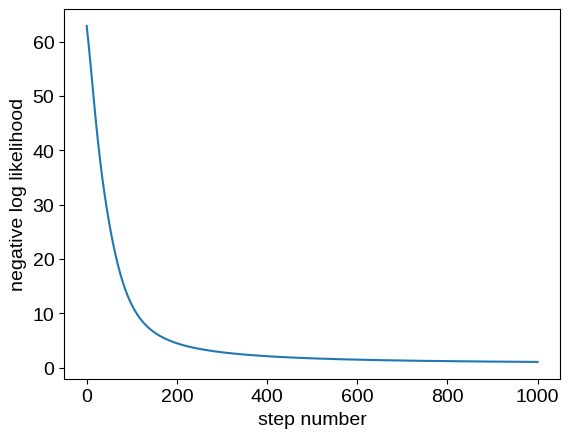
for i in range(1001):
    loss_val, grads = loss_grad_fn(params)
    losses.append(loss_val)
    updates, opt_state = tx.update(grads, opt_state)
    params = optax.apply_updates(params, updates)

plt.plot(losses)
plt.ylabel("negative log likelihood")
_ = plt.xlabel("step number")

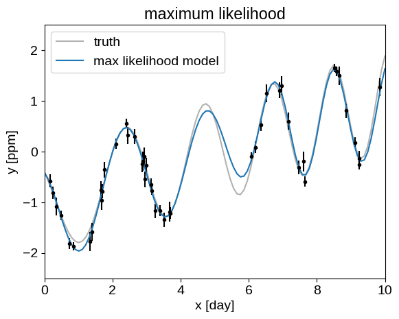
Our Module defined above also returns the conditional predictions, that we can compare to the true model:

pred = model.apply(params, t, yerr, y, true_t)[1]

plt.plot(true_t, true_y, "k", lw=1.5, alpha=0.3, label="truth")
plt.errorbar(t, y, yerr=yerr, fmt=".k", capsize=0)
plt.plot(true_t, pred, label="max likelihood model")
plt.xlabel("x [day]")
plt.ylabel("y [ppm]")
plt.xlim(0, 10)
plt.ylim(-2.5, 2.5)
plt.legend()
_ = plt.title("maximum likelihood")

Sampling with numpyro

Perhaps we’re not satisfied with just a point estimate of our hyperparameters and we want to instead compute posterior expectations. One tool for doing that is numpyro, which offers Markov chain Monte Carlo (MCMC) and variational inference methods. As a demonstration, here’s how we would set up the model from above and run MCMC in numpyro:

import numpyro
import numpyro.distributions as dist
from numpyro.infer import MCMC, NUTS

prior_sigma = 5.0


def numpyro_model(t, yerr, y=None):
    mean = numpyro.sample("mean", dist.Normal(0.0, prior_sigma))
    jitter = numpyro.sample("jitter", dist.HalfNormal(prior_sigma))

    sigma1 = numpyro.sample("sigma1", dist.HalfNormal(prior_sigma))
    rho1 = numpyro.sample("rho1", dist.HalfNormal(prior_sigma))
    tau = numpyro.sample("tau", dist.HalfNormal(prior_sigma))
    kernel1 = sigma1**2 * kernels.ExpSquared(tau) * kernels.Cosine(rho1)

    sigma2 = numpyro.sample("sigma2", dist.HalfNormal(prior_sigma))
    rho2 = numpyro.sample("rho2", dist.HalfNormal(prior_sigma))
    kernel2 = sigma2**2 * kernels.Matern32(rho2)

    kernel = kernel1 + kernel2
    gp = GaussianProcess(kernel, t, diag=yerr**2 + jitter, mean=mean)
    numpyro.sample("gp", gp.numpyro_dist(), obs=y)

    if y is not None:
        numpyro.deterministic("pred", gp.condition(y, true_t).gp.loc)


nuts_kernel = NUTS(numpyro_model, dense_mass=True, target_accept_prob=0.9)
mcmc = MCMC(
    nuts_kernel,
    num_warmup=1000,
    num_samples=1000,
    num_chains=2,
    progress_bar=False,
)
rng_key = jax.random.PRNGKey(34923)

/tmp/ipykernel_5000/1709763210.py:30: UserWarning: There are not enough devices to run parallel chains: expected 2 but got 1. Chains will be drawn sequentially. If you are running MCMC in CPU, consider using `numpyro.set_host_device_count(2)` at the beginning of your program. You can double-check how many devices are available in your system using `jax.local_device_count()`.
  mcmc = MCMC(

%%time
mcmc.run(rng_key, t, yerr, y=y)
samples = mcmc.get_samples()
pred = samples["pred"].block_until_ready()  # Blocking to get timing right

CPU times: user 51.6 s, sys: 15 s, total: 1min 6s
Wall time: 37.3 s

When running iterative methods like MCMC, it’s always a good idea to check some convergence diagnostics. For that task, let’s use ArviZ:

import arviz as az

data = az.from_numpyro(mcmc)
az.summary(data, var_names=[v for v in data.posterior.data_vars if v != "pred"])

	mean	sd	hdi_3%	hdi_97%	mcse_mean	mcse_sd	ess_bulk	ess_tail	r_hat
jitter	0.003	0.004	0.000	0.009	0.000	0.000	1228.0	746.0	1.00
mean	-0.027	1.486	-2.973	2.677	0.054	0.048	950.0	792.0	1.00
rho1	2.276	0.650	1.782	2.898	0.050	0.035	547.0	202.0	1.00
rho2	7.351	3.128	1.764	12.674	0.089	0.063	1171.0	1039.0	1.00
sigma1	1.053	0.489	0.461	1.913	0.019	0.014	1205.0	723.0	1.01
sigma2	1.734	1.006	0.412	3.677	0.036	0.026	883.0	978.0	1.00
tau	2.206	0.998	0.612	4.014	0.042	0.030	473.0	349.0	1.01

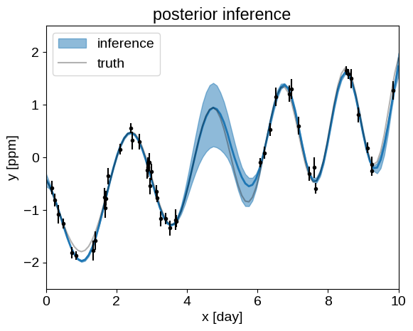
And, finally we can plot our posterior inferences of the conditional process, compared to the true model:

q = np.percentile(pred, [5, 50, 95], axis=0)
plt.fill_between(true_t, q[0], q[2], color="C0", alpha=0.5, label="inference")
plt.plot(true_t, q[1], color="C0", lw=2)
plt.plot(true_t, true_y, "k", lw=1.5, alpha=0.3, label="truth")

plt.errorbar(t, y, yerr=yerr, fmt=".k", capsize=0)
plt.xlabel("x [day]")
plt.ylabel("y [ppm]")
plt.xlim(0, 10)
plt.ylim(-2.5, 2.5)
plt.legend()
_ = plt.title("posterior inference")