Kernel Transforms#

tinygp is designed to make it easy to implement new kernels (see Custom Kernels for an example), but a particular set of customizations that tinygp supports with a high-level interface are coordinate transforms. The basic idea here is that you may want to pass your input coordinates through a linear or non-linear transformation before evaluating one of the standard kernels in that transformed space. This is particularly useful for multivariate inputs where, for example, you may want to capture the different units, or prior covariances between dimensions.

Example: Deep kernel lerning#

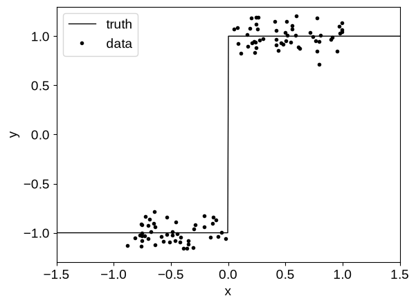
The Deep Kernel Learning model is an example of a more complicated kernel transform, and since tinygp integrates well with libraries like flax (see Modeling Frameworks) the implementation of such a model is fairly straightforward. To demonstrate, let’s start by sampling a simulated dataset from a step function, a model that a GP would typically struggle to model:

import numpy as np
import matplotlib.pyplot as plt

random = np.random.default_rng(567)

noise = 0.1

x = np.sort(random.uniform(-1, 1, 100))
y = 2 * (x > 0) - 1 + random.normal(0.0, noise, len(x))
t = np.linspace(-1.5, 1.5, 500)

plt.plot(t, 2 * (t > 0) - 1, "k", lw=1, label="truth")
plt.plot(x, y, ".k", label="data")
plt.xlim(-1.5, 1.5)
plt.ylim(-1.3, 1.3)
plt.xlabel("x")
plt.ylabel("y")
_ = plt.legend()

../_images/b9e158e0a528088cbda414e24a07aaf5f76eafcf431e9bceaf29f98b21d26dfd.png

Then we will fit this model using a model similar to the one described in Optimization with flax & optax, except our kernel will include a custom tinygp.kernels.Transform that will pass the input coordinates through a (small) neural network before passing them into a tinygp.kernels.Matern32 kernel. Otherwise, the model and optimization procedure are similar to the ones used in Optimization with flax & optax.

We compare the performance of the Deep Matern-3/2 kernel (a tinygp.kernels.Matern32 kernel, with custom neural network transform) to the performance of the same kernel without the transform. The untransformed model doesn’t have the capacity to capture our simulated step function, but our transformed model does. In our transformed model, the hyperparameters of our kernel now include the weights of our neural network transform, and we learn those simultaneously with the length scale and amplitude of the Matern32 kernel.

import jax
import optax
import jax.numpy as jnp
import flax.linen as nn
from flax.linen.initializers import zeros
from tinygp import kernels, transforms, GaussianProcess

class Transformer(nn.Module):
    """A small neural network used to non-linearly transform the input data"""

    @nn.compact
    def __call__(self, x):
        x = nn.Dense(features=15)(x)
        x = nn.relu(x)
        x = nn.Dense(features=10)(x)
        x = nn.relu(x)
        x = nn.Dense(features=1)(x)
        return x


class DeepLoss(nn.Module):
    @nn.compact
    def __call__(self, x, y, t):
        # Set up a typical Matern-3/2 kernel
        log_sigma = self.param("log_sigma", zeros, ())
        log_rho = self.param("log_rho", zeros, ())
        log_jitter = self.param("log_jitter", zeros, ())
        base_kernel = jnp.exp(2 * log_sigma) * kernels.Matern32(jnp.exp(log_rho))

        # Define a custom transform to pass the input coordinates through our
        # `Transformer` network from above
        # Note: with recent version of flax, you can't directly vmap modules,
        # but we can get around that by explicitly constructing the init and
        # apply functions. Ref:
        # https://flax.readthedocs.io/en/latest/advanced_topics/lift.html
        transform = Transformer()
        transform_params = self.param("transform", transform.init, x[:1])
        apply_fn = lambda x: transform.apply(transform_params, x)
        kernel = transforms.Transform(apply_fn, base_kernel)

        # Evaluate and return the GP negative log likelihood as usual with the
        # transformed features
        gp = GaussianProcess(
            kernel, x[:, None], diag=noise**2 + jnp.exp(2 * log_jitter)
        )
        log_prob, gp_cond = gp.condition(y, t[:, None])

        # We return the loss, the conditional mean and variance, and the
        # transformed input parameters
        return (
            -log_prob,
            (gp_cond.loc, gp_cond.variance),
            (transform(x[:, None]), transform(t[:, None])),
        )


# Define and train the model
def loss_func(model):
    def loss(params):
        return model.apply(params, x, y, t)[0]

    return loss


models_list, params_list = [], []
loss_vals = {}
# Plot the results and compare to the true model
fig, ax = plt.subplots(ncols=2, sharey=True, figsize=(9, 3))
for it, (model_name, model) in enumerate(
    zip(
        ["Deep", "Matern32"],
        [DeepLoss(), Matern32Loss()],
    )
):
    loss_vals[it] = []
    params = model.init(jax.random.PRNGKey(1234), x, y, t)
    tx = optax.sgd(learning_rate=1e-4)
    opt_state = tx.init(params)

    loss = loss_func(model)
    loss_grad_fn = jax.jit(jax.value_and_grad(loss))
    for i in range(1000):
        loss_val, grads = loss_grad_fn(params)
        updates, opt_state = tx.update(grads, opt_state)
        params = optax.apply_updates(params, updates)
        loss_vals[it].append(loss_val)

    mu, var = model.apply(params, x, y, t)[1]
    ax[it].plot(t, 2 * (t > 0) - 1, "k", lw=1, label="truth")
    ax[it].plot(x, y, ".k", label="data")
    ax[it].plot(t, mu)
    ax[it].fill_between(
        t, mu + np.sqrt(var), mu - np.sqrt(var), alpha=0.5, label="model"
    )
    ax[it].set_xlim(-1.5, 1.5)
    ax[it].set_ylim(-1.3, 1.3)
    ax[it].set_xlabel("x")
    ax[it].set_ylabel("y")
    ax[it].set_title(model_name)
    _ = ax[it].legend()

    models_list.append(model)
    params_list.append(params)

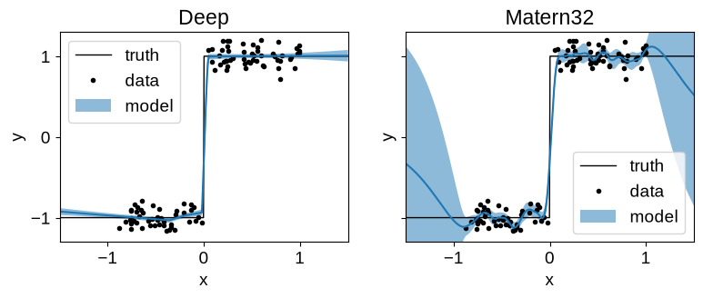
../_images/050155eabbce082b35515711234915f5bdf4e7f2a519ac7c8ec2dc052b9bb27d.png

The untransformed Matern32 model suffers from over-smoothing at the discontinuity, and poor extrapolation performance. The Deep model extrapolates well and captures the discontinuity reliably.

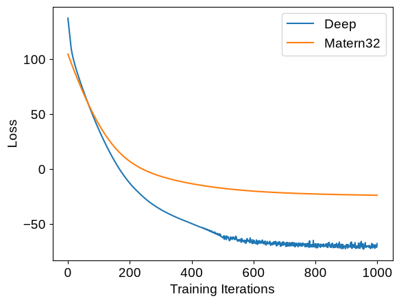
We can compare the training loss (negative log likelihood) traces for these two models:

fig = plt.plot()
plt.plot(loss_vals[0], label="Deep")
plt.plot(loss_vals[1], label="Matern32")
plt.ylabel("Loss")
plt.xlabel("Training Iterations")
_ = plt.legend()

../_images/0fc5de42b57a4c61269f01426ca299f54a1d7d63fa1682ceaa36fff4ff8ed066.png

To inspect what the transformed model is doing under the hood, we can plot the functional form of the transformation, as well as the transformed values of our input coordinates:

x_transform, t_transform = models_list[0].apply(params_list[0], x, y, t)[2]

fig = plt.figure()
plt.plot(t, t_transform, "k")
plt.xlim(-1.5, 1.5)
plt.ylim(-1.3, 1.3)
plt.xlabel("input data; x")
plt.ylabel("transformed data; x'")

fig, ax = plt.subplots(ncols=2, sharey=True, figsize=(9, 3))
for it, (fig_title, feature_input, x_label) in enumerate(
    zip(["Input Data", "Transformed Data"], [x, x_transform], ["x", "x'"])
):
    ax[it].plot(feature_input, y, ".k")
    ax[it].set_xlim(-1.5, 1.5)
    ax[it].set_ylim(-1.3, 1.3)
    ax[it].set_title(fig_title)
    ax[it].set_xlabel(x_label)
    ax[it].set_ylabel("y")

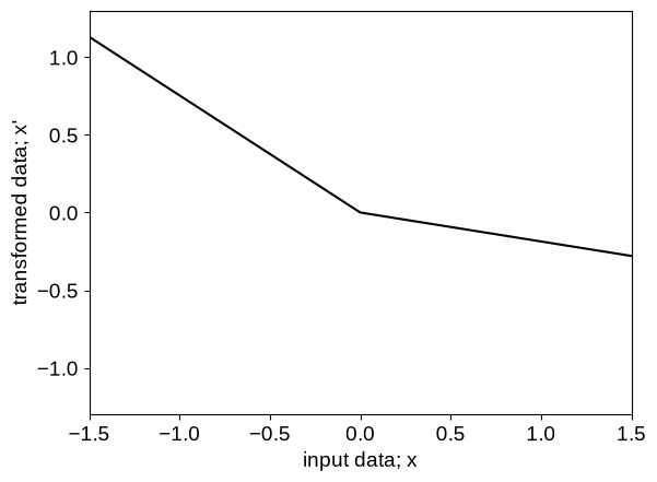
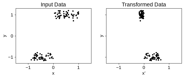
../_images/93ba411f3fa60fdb5a4eb86d3c658f806fe7c840568e2a666263b3456cd0e9ef.png

../_images/4b9f6461704e2070590a454a9d20efd4c330f602ff16a07e66aec53008c09b30.png

The neural network transforms the input feature into a step function like data (as shown in the figures above) before feeding to the base kernel, making it better suited than the baseline model for this data.

Kernel Transforms

Contents

Kernel Transforms#

Example: Deep kernel lerning#