Non-Gaussian Likelihoods#
In this tutorial, we demonstrate how tinygp can be used in combination with non-Gaussian observation models.
The basic idea is that your tinygp model can be a middle layer in your probabilistic model; it doesn’t just have to be at the bottom.
One issue with this is that the marginalization over process realizations will no longer be analytic, so you’ll need to marginalize numerically using Markov chain Monte Carlo (MCMC) or variational inference (VI).
Since tinygp doesn’t include any built-in inference methods you’ll need to use a different package, but luckily there are lots of good tools that exist!
In this case, we’ll use numpyro.
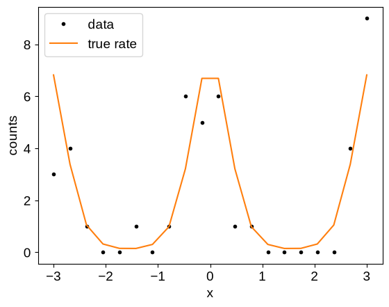
As our test case, we’ll look at counts data with a Poisson observation model where the underlying log-rate is modeled by a Gaussian process (also known as a Cox process). To begin, let’s simulate some data:
import matplotlib.pyplot as plt
import numpy as np

random = np.random.default_rng(203618)
x = np.linspace(-3, 3, 20)
true_log_rate = 2 * np.cos(2 * x)
y = random.poisson(np.exp(true_log_rate))
plt.plot(x, y, ".k", label="data")
plt.plot(x, np.exp(true_log_rate), "C1", label="true rate")
plt.legend(loc=2)
plt.xlabel("x")
_ = plt.ylabel("counts")
Markov chain Monte Carlo (MCMC)#
Then we set up the model in numpyro and run the MCMC, following the example in Sampling with numpyro.
The main difference here is that we’re using MCMC to marginalize over GP realizations (that is encoded in the following by the fact that the log_rate parameter doesn’t have the obs=... argument set), instead of analytically marginalizing.
import jax
import jax.numpy as jnp
import numpyro
import numpyro.distributions as dist

from tinygp import GaussianProcess, kernels

jax.config.update("jax_enable_x64", True)


def model(x, y=None):
    # The parameters of the GP model
    mean = numpyro.sample("mean", dist.Normal(0.0, 2.0))
    sigma = numpyro.sample("sigma", dist.HalfNormal(3.0))
    rho = numpyro.sample("rho", dist.HalfNormal(10.0))

    # Set up the kernel and GP objects
    kernel = sigma**2 * kernels.Matern52(rho)
    gp = GaussianProcess(kernel, x, diag=1e-5, mean=mean)

    # This parameter has shape (num_data,) and it encodes our beliefs about
    # the process rate in each bin
    log_rate = numpyro.sample("log_rate", gp.numpyro_dist())

    # Finally, our observation model is Poisson
    numpyro.sample("obs", dist.Poisson(jnp.exp(log_rate)), obs=y)


# Run the MCMC
nuts_kernel = numpyro.infer.NUTS(model, target_accept_prob=0.9)
mcmc = numpyro.infer.MCMC(
    nuts_kernel,
    num_warmup=1000,
    num_samples=1000,
    num_chains=2,
    progress_bar=False,
)
rng_key = jax.random.PRNGKey(55873)
mcmc.run(rng_key, x, y=y)
samples = mcmc.get_samples()
/tmp/ipykernel_1111/4167427703.py:31: UserWarning: There are not enough devices to run parallel chains: expected 2 but got 1. Chains will be drawn sequentially. If you are running MCMC in CPU, consider using `numpyro.set_host_device_count(2)` at the beginning of your program. You can double-check how many devices are available in your system using `jax.local_device_count()`.
  mcmc = numpyro.infer.MCMC(
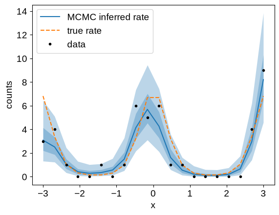
We can summarize the MCMC results by plotting our inferred model (here we’re showing the 1- and 2-sigma credible regions), and compare it to the known ground truth:
q = np.percentile(samples["log_rate"], [5, 25, 50, 75, 95], axis=0)
plt.plot(x, np.exp(q[2]), color="C0", label="MCMC inferred rate")
plt.fill_between(x, np.exp(q[0]), np.exp(q[-1]), alpha=0.3, lw=0, color="C0")
plt.fill_between(x, np.exp(q[1]), np.exp(q[-2]), alpha=0.3, lw=0, color="C0")
plt.plot(x, np.exp(true_log_rate), "--", color="C1", label="true rate")
plt.plot(x, y, ".k", label="data")
plt.legend(loc=2)
plt.xlabel("x")
_ = plt.ylabel("counts")
Stochastic variational inference (SVI)#
The above results look good and didn’t take long to run, but if we had more data the runtime could become prohibitive, since the number of parameters scales with the sizegreater_than the dataset.
In cases like this, we can compute the relevant expectations using stochastic variational inference (SVI) instead of MCMC.
Here’s one way that you could set up such a model using tinygp and numpyro:
def model(x, y=None):
    # The parameters of the GP model
    mean = numpyro.param("mean", jnp.zeros(()))
    sigma = numpyro.param("sigma", jnp.ones(()), constraint=dist.constraints.positive)
    rho = numpyro.param("rho", 2 * jnp.ones(()), constraint=dist.constraints.positive)

    # Set up the kernel and GP objects
    kernel = sigma**2 * kernels.Matern52(rho)
    gp = GaussianProcess(kernel, x, diag=1e-5, mean=mean)

    # This parameter has shape (num_data,) and it encodes our beliefs about
    # the process rate in each bin
    log_rate = numpyro.sample("log_rate", gp.numpyro_dist())

    # Finally, our observation model is Poisson
    numpyro.sample("obs", dist.Poisson(jnp.exp(log_rate)), obs=y)


def guide(x, y=None):
    mu = numpyro.param(
        "log_rate_mu", jnp.zeros_like(x) if y is None else jnp.log(y + 1)
    )
    sigma = numpyro.param(
        "log_rate_sigma",
        jnp.ones_like(x),
        constraint=dist.constraints.positive,
    )
    numpyro.sample("log_rate", dist.Independent(dist.Normal(mu, sigma), 1))


optim = numpyro.optim.Adam(0.01)
svi = numpyro.infer.SVI(model, guide, optim, numpyro.infer.Trace_ELBO(10))
results = svi.run(jax.random.PRNGKey(55873), 3000, x, y=y, progress_bar=False)
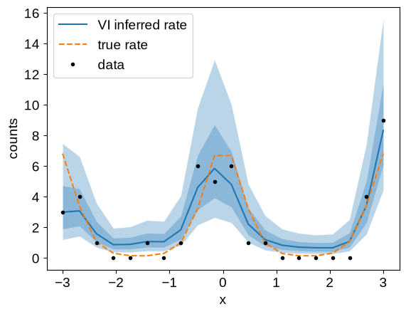
As above, we can plot our inferred conditional model and compare it to the ground truth:
mu = results.params["log_rate_mu"]
sigma = results.params["log_rate_sigma"]
plt.plot(x, np.exp(mu), color="C0", label="VI inferred rate")
plt.fill_between(
    x,
    np.exp(mu - 2 * sigma),
    np.exp(mu + 2 * sigma),
    alpha=0.3,
    lw=0,
    color="C0",
)
plt.fill_between(x, np.exp(mu - sigma), np.exp(mu + sigma), alpha=0.3, lw=0, color="C0")
plt.plot(x, np.exp(true_log_rate), "--", color="C1", label="true rate")
plt.plot(x, y, ".k", label="data")
plt.legend(loc=2)
plt.xlabel("x")
_ = plt.ylabel("counts")